CS 25.331 Symmetric manoeuvring conditions

ED Decision 2016/010/R

(See AMC 25.331)

(a) Procedure. For the analysis of the manoeuvring flight conditions specified in sub-paragraphs (b) and (c) of this paragraph, the following provisions apply:

(1) Where sudden displacement of a control is specified, the assumed rate of control surface displacement may not be less than the rate that could be applied by the pilot through the control system.

(2) In determining elevator angles and chordwise load distribution in the manoeuvring conditions of sub-paragraphs (b) and (c) of this paragraph, the effect of corresponding pitching velocities must be taken into account. The in-trim and out-of-trim flight conditions specified in CS 25.255 must be considered.

(b) Manoeuvring balanced conditions. Assuming the aeroplane to be in equilibrium with zero pitching acceleration, the manoeuvring conditions A through I on the manoeuvring envelope in CS 25.333(b) must be investigated.

(c) Manoeuvring pitching conditions. The following conditions must be investigated:

(1) Maximum pitch control displacement at V_A. The aeroplane is assumed to be flying in steady level flight (point A1, CS 25.333(b)) and the cockpit pitch control is suddenly moved to obtain extreme nose up pitching acceleration. In defining the tail load, the response of the aeroplane must be taken into account. Aeroplane loads which occur subsequent to the time when normal acceleration at the c.g. exceeds the positive limit manoeuvring load factor (at point A2 in CS 25.333(b)), or the resulting tailplane normal load reaches its maximum, whichever occurs first, need not be considered (See AMC 25.331(c)(1)).

(2) Checked manoeuvre between V_A and V_D. Nose up checked pitching manoeuvres must be analysed in which the positive limit load factor prescribed in CS 25.337 is achieved. As a separate condition, nose down checked pitching manoeuvres must be analysed in which a limit load factor of 0 is achieved. In defining the aeroplane loads the cockpit pitch control motions described in sub-paragraphs (i), (ii), (iii) and (iv) of this paragraph must be used:

(See AMC 25.331(c)(2))

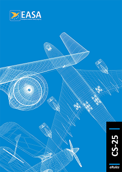
(i) The aeroplane is assumed to be flying in steady level flight at any speed between V_A and V_D and the cockpit pitch control is moved in accordance with the following formula:

where:

δ1 =  the maximum available displacement of the cockpit pitch control in the initial direction, as limited by the control system stops, control surface stops, or by pilot effort in accordance with CS 25.397(b);

δ(t) = the displacement of the cockpit pitch control as a function of time. In the initial direction δ(t) is limited to δ₁. In the reverse direction, δ(t) may be truncated at the maximum available displacement of the cockpit pitch control as limited by the control system stops, control surface stops, or by pilot effort in accordance with CS 25.397(b);

t_max = 3π/2ω;

ω =  the circular frequency (radians/second) of the control deflection taken equal to the undamped natural frequency of the short period rigid mode of the aeroplane, with active control system effects included where appropriate; but not less than:

where:

V =  the speed of the aeroplane at entry to the manoeuvre.

V_A =  the design manoeuvring speed prescribed in CS 25.335(c)

(ii) For nose-up pitching manoeuvres the complete cockpit pitch control displacement history may be scaled down in amplitude to the extent just necessary to ensure that the positive limit load factor prescribed in CS 25.337 is not exceeded. For nose-down pitching manoeuvres the complete cockpit control displacement history may be scaled down in amplitude to the extent just necessary to ensure that the normal acceleration at the c.g. does not go below 0g.

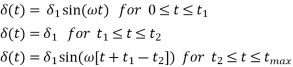
(iii) In addition, for cases where the aeroplane response to the specified cockpit pitch control motion does not achieve the prescribed limit load factors then the following cockpit pitch control motion must be used:

where:

t₁   = π/2ω

t₂   = t₁ + ∆t

t_max = t₂ + π/ω;

∆t  = the minimum period of time necessary to allow the prescribed limit load factor to be achieved in the initial direction, but it need not exceed five seconds (see figure below).

(iv) In cases where the cockpit pitch control motion may be affected by inputs from systems (for example, by a stick pusher that can operate at high load factor as well as at 1g) then the effects of those systems must be taken into account.

(v) Aeroplane loads that occur beyond the following times need not be considered:

(A) For the nose-up pitching manoeuvre, the time at which the normal acceleration at the c.g. goes below 0g;

(B) For the nose-down pitching manoeuvre, the time at which the normal acceleration at the c.g. goes above the positive limit load factor prescribed in CS 25.337;

(C)  t_max.

[Amdt 25/13]

[Amdt 25/18]

AMC 25.331(c)(1) Maximum pitch control displacement at V_A

ED Decision 2013/010/R

The physical limitations of the aircraft from the cockpit pitch control device to the control surface deflection, such as control stops position, maximum power and displacement rate of the servo controls, and control law limiters, may be taken into account.

[Amdt 25/13]

AMC 25.331(c)(2) Checked manoeuvre between V_A and V_D

ED Decision 2013/010/R

The physical limitations of the aircraft from the cockpit pitch control device to the control surface deflection, such as control stops position, maximum power and displacement rate of the servo controls, and control law limiters, may be taken into account.

For aeroplanes equipped with electronic flight controls, where the motion of the control surfaces does not bear a direct relationship to the motion of the cockpit control devices, the circular frequency of the movement of the cockpit control ‘ω’ shall be varied by a reasonable amount to establish the effect of the input period and amplitude on the resulting aeroplane loads. This variation is intended to verify that there is no large and rapid increase in aeroplane loads.

[Amdt 25/13]

CS 25.333 Flight manoeuvring envelope

ED Decision 2016/010/R

(See AMC 25.333)

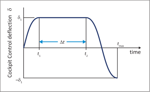
(a) General. The strength requirements must be met at each combination of airspeed and load factor on and within the boundaries of the representative manoeuvring envelope (V-n diagram) of sub-paragraph (b) of this paragraph. This envelope must also be used in determining the aeroplane structural operating limitations as specified in CS 25.1501.

(b) Manoeuvring envelope (See AMC 25.333(b))

[Amdt 25/11]

[Amdt 25/13]

[Amdt 25/18]

AMC 25.333(b) Manoeuvring envelope

ED Decision 2013/010/R

For the calculation of structural design speeds, the stalling speeds V_s0 and V_s1 should be taken to be the 1-g stalling speeds in the appropriate flap configuration. This structural interpretation of stalling speed should be used in connection with the paragraphs CS 25.333(b), CS 25.335, CS 25.335(c)(d)(e), CS 25.479(a), and CS 25.481(a)(1).

[Amdt 25/13]

CS 25.335 Design airspeeds

ED Decision 2016/010/R

(See AMC 25.335)

The selected design airspeeds are equivalent airspeeds (EAS). Estimated values of V_S0 and V_S1 must be conservative.

(a) Design cruising speed, V_C. For V_C, the following apply:

(1) The minimum value of V_C must be sufficiently greater than V_B to provide for inadvertent speed increases likely to occur as a result of severe atmospheric turbulence.

(2) Except as provided in sub-paragraph 25.335(d)(2), V_C may not be less than V_B + 1·32 U_ref (with U_ref as specified in sub-paragraph 25.341(a)(5)(i). However, V_C need not exceed the maximum speed in level flight at maximum continuous power for the corresponding altitude.

(3) At altitudes where V_D is limited by Mach number, V_C may be limited to a selected Mach number. (See CS 25.1505.)

(b) Design dive speed, V_D. V_D must be selected so that V_C/M_C is not greater than 0·8 V_D/M_D, or so that the minimum speed margin between V_C/M_C and V_D/M_D is the greater of the following values:

(1) (i) For aeroplanes not equipped with a high speed protection function: From an initial condition of stabilised flight at V_C/M_C, the aeroplane is upset, flown for 20 seconds along a flight path 7·5° below the initial path, and then pulled up at a load factor of 1·5 g (0·5 g acceleration increment). The speed increase occurring in this manoeuvre may be calculated if reliable or conservative aerodynamic data issued. Power as specified in CS 25.175(b)(1)(iv) is assumed until the pullup is initiated, at which time power reduction and the use of pilot controlled drag devices may be assumed;

(ii) For aeroplanes equipped with a high speed protection function: In lieu of subparagraph (b)(1)(i), the speed increase above V_C/M_C resulting from the greater of the following manoeuvres must be established:

(A) From an initial condition of stabilised flight at V_C/M_C, the aeroplane is upset so as to take up a new flight path 7.5° below the initial path. Control application, up to full authority, is made to try and maintain this new flight path. Twenty seconds after achieving the new flight path, manual recovery is made at a load factor of 1.5 g (0.5 g acceleration increment), or such greater load factor that is automatically applied by the system with the pilot’s pitch control neutral. The speed increase occurring in this manoeuvre may be calculated if reliable or conservative aerodynamic data is used. Power as specified in CS 25.175(b)(1)(iv) is assumed until recovery is made, at which time power reduction and the use of pilot controlled drag devices may be assumed.

(B) From a speed below V_C/M_C, with power to maintain stabilised level flight at this speed, the aeroplane is upset so as to accelerate through V_C/M_C at a flight path 15° below the initial path (or at the steepest nose down attitude that the system will permit with full control authority if less than 15°). Pilot controls may be in neutral position after reaching V_C/M_C and before recovery is initiated. Recovery may be initiated 3 seconds after operation of high speed, attitude, or other alerting system by application of a load factor of 1.5 g (0.5 g acceleration increment), or such greater load factor that is automatically applied by the system with the pilot’s pitch control neutral. Power may be reduced simultaneously. All other means of decelerating the aeroplane, the use of which is authorised up to the highest speed reached in the manoeuvre, may be used. The interval between successive pilot actions must not be less than 1 second (See AMC 25.335(b)(1)(ii)).

(2) The minimum speed margin must be enough to provide for atmospheric variations (such as horizontal gusts, and penetration of jet streams and cold fronts) and for instrument errors and airframe production variations. These factors may be considered on a probability basis. The margin at altitude where M_C is limited by compressibility effects must not be less than 0.07M unless a lower margin is determined using a rational analysis that includes the effects of any automatic systems. In any case, the margin may not be reduced to less than 0.05M. (See AMC 25.335(b)(2))

(c) Design manoeuvring speed, V_A. For V_A, the following apply:

(1) V_A may not be less than VS1 √n where –

(i) n is the limit positive manoeuvring load factor at V_C; and

(ii) V_S1 is the stalling speed with wing-flaps retracted.

(2) V_A and V_S must be evaluated at the design weight and altitude under consideration.

(3) V_A need not be more than V_C or the speed at which the positive C_Nmax curve intersects the positive manoeuvre load factor line, whichever is less.

(d) Design speed for maximum gust intensity, V_B.

(1) V_B may not be less than

where –

V_sl   = the 1-g stalling speed based on C_NAmax with the flaps retracted at the particular weight under consideration;

C_NAmax = the maximum aeroplane normal force coefficient;

V_c   = design cruise speed (knots equivalent airspeed);

U_ref = the reference gust velocity (feet per second equivalent airspeed) from CS 25.341(a)(5)(i);

w   = average wing loading (pounds per square foot) at the particular weight under consideration.

K_g   = 

µ    = 

ρ    = density of air (slugs/ft³);

c    = mean geometric chord of the wing (feet);

g    = acceleration due to gravity (ft/sec²);

a    = slope of the aeroplane normal force coefficient curve, C_NA per radian;

(2) At altitudes where V_c is limited by Mach number –

(i) V_B may be chosen to provide an optimum margin between low and high speed buffet boundaries; and,

(ii) V_B need not be greater than V_C.

(e) Design wing-flap speeds, V_F. For V_F, the following apply:

(1) The design wing-flap speed for each wing-flap position (established in accordance with CS 25.697(a)) must be sufficiently greater than the operating speed recommended for the corresponding stage of flight (including balked landings) to allow for probable variations in control of airspeed and for transition from one wing-flap position to another.

(2) If an automatic wing-flap positioning or load limiting device is used, the speeds and corresponding wing-flap positions programmed or allowed by the device may be used.

(3) V_F may not be less than –

(i) 1·6 V_S1 with the wing-flaps in take-off position at maximum take-off weight;

(ii) 1·8 V_S1 with the wing-flaps in approach position at maximum landing weight; and

(iii) 1·8 V_S0 with the wing-flaps in landing position at maximum landing weight.

(f) Design drag device speeds, V_DD. The selected design speed for each drag device must be sufficiently greater than the speed recommended for the operation of the device to allow for probable variations in speed control. For drag devices intended for use in high speed descents, V_DD may not be less than V_D. When an automatic drag device positioning or load limiting means is used, the speeds and corresponding drag device positions programmed or allowed by the automatic means must be used for design.

[Amdt 25/13]

[Amdt 25/18]

AMC 25.335(b)(1)(ii) Design Dive Speed - High speed protection function

ED Decision 2013/010/R

In any failure condition affecting the high speed protection function, the conditions as defined in CS 25.335(b)(1)(ii) still remain applicable.

It implies that a specific value, which may be different from the V_D/M_D value in normal configuration, has to be associated with this failure condition for the definition of loads related to V_D/M_D as well as for the justification to CS 25.629. However, the strength and speed margin required will depend on the probability of this failure condition, according to the criteria of CS 25.302.

Alternatively, the operating speed V_MO/M_MO may be reduced to a value that maintains a speed margin between V_MO/M_MO and V_D/M_D that is consistent with showing compliance with CS 25.335(b)(1)(ii) without the benefit of the high speed protection system, provided that:

(a) Any failure of the high speed protection system that would affect the design dive speed determination is shown to be Remote;

(b) Failures of the system must be announced to the pilots, and:

(c) Aeroplane flight manual instructions should be provided that reduce the maximum operating speeds, V_MO/M_MO.

[Amdt 25/13]

AMC 25.335(b)(2) Design Dive Speed

ED Decision 2006/005/R

1. PURPOSE. This AMC sets forth an acceptable means, but not the only means, of demonstrating compliance with the provisions of CS-25 related to the minimum speed margin between design cruise speed and design dive speed.

2. RELATED CERTIFICATION SPECIFICATIONS. CS 25.335 "Design airspeeds".

3. BACKGROUND. CS 25.335(b) requires the design dive speed, V_D, of the aeroplane to be established so that the design cruise speed is no greater than 0.8 times the design dive speed, or that it be based on an upset criterion initiated at the design cruise speed, V_C. At altitudes where the cruise speed is limited by compressibility effects, CS 25.335(b)(2) requires the margin to be not less than 0.05 Mach. Furthermore, at any altitude, the margin must be great enough to provide for atmospheric variations (such as horizontal gusts and the penetration of jet streams), instrument errors, and production variations. This AMC provides a rational method for considering the atmospheric variations.

4. DESIGN DIVE SPEED MARGIN DUE TO ATMOSPHERIC VARIATIONS.

a. In the absence of evidence supporting alternative criteria, compliance with CS 25.335(b)(2) may be shown by providing a margin between V_C/M_C and V_D/M_D sufficient to provide for the following atmospheric conditions:

(1) Encounter with a Horizontal Gust. The effect of encounters with a substantially headon gust, assumed to act at the most adverse angle between 30 degrees above and 30 degrees below the flight path, should be considered. The gust velocity should be 15.2 m/s (50 fps) in equivalent airspeed (EAS) at altitudes up to 6096 m (20,000 feet). At altitudes above 6096 m (20,000 feet) the gust velocity may be reduced linearly from 15.2 m/s (50 fps) in EAS at 6096 m (20,000 feet) to 7.6 m/s (25 fps) in EAS at 15240 m (50,000 feet), above which the gust velocity is considered to be constant. The gust velocity should be assumed to build up in not more than 2 seconds and last for 30 seconds.

(2) Entry into Jetstreams or Regions of High Windshear.

(i) Conditions of horizontal and vertical windshear should be investigated taking into account the windshear data of this paragraph which are world-wide extreme values.

(ii) Horizontal windshear is the rate of change of horizontal wind speed with horizontal distance. Encounters with horizontal windshear change the aeroplane apparent head wind in level flight as the aeroplane traverses into regions of changing wind speed. The horizontal windshear region is assumed to have no significant vertical gradient of wind speed.

(iii) Vertical windshear is the rate of change of horizontal wind speed with altitude. Encounters with windshear change the aeroplane apparent head wind as the aeroplane climbs or descends into regions of changing wind speed. The vertical windshear region changes slowly so that temporal or spatial changes in the vertical windshear gradient are assumed to have no significant affect on an aeroplane in level flight.

(iv) With the aeroplane at V_C/M_C within normal rates of climb and descent, the most extreme condition of windshear that it might encounter, according to available meteorological data, can be expressed as follows:

(A) Horizontal Windshear. The jet stream is assumed to consist of a linear shear of 3.6 KTAS/NM over a distance of 25 NM or of 2.52 KTAS/NM over a distance of 50 NM or of 1.8 KTAS/NM over a distance of 100 NM, whichever is most severe.

(B) Vertical Windshear. The windshear region is assumed to have the most severe of the following characteristics and design values for windshear intensity and height band. As shown in Figure 1, the total vertical thickness of the windshear region is twice the height band so that the windshear intensity specified in Table 1 applies to a vertical distance equal to the height band above and below the reference altitude. The variation of horizontal wind speed with altitude in the windshear region is linear through the height band from zero at the edge of the region to a strength at the reference altitude determined by the windshear intensity multiplied by the height band. Windshear intensity varies linearly between the reference altitudes in Table 1.

Figure 1 - Windshear Region

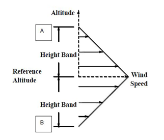
Note: The analysis should be conducted by separately descending from point “A” and climbing from point “B” into initially increasing headwind.

Table 1 - Vertical Windshear Intensity Characteristics

(v) The entry of the aeroplane into horizontal and vertical windshear should be treated as separate cases. Because the penetration of these large scale phenomena is fairly slow, recovery action by the pilot is usually possible. In the case of manual flight (i.e., when flight is being controlled by inputs made by the pilot), the aeroplane is assumed to maintain constant attitude until at least 3 seconds after the operation of the overspeed warning device, at which time recovery action may be started by using the primary aerodynamic controls and thrust at a normal acceleration of 1.5g, or the maximum available, whichever is lower.

b. At altitudes where speed is limited by Mach number, a speed margin of .07 Mach between M_C and M_D is considered sufficient without further investigation.

[Amdt 25/2]

CS 25.337 Limit manoeuvring load factors

ED Decision 2003/2/RM

(See AMC 25.337)

(a) Except where limited by maximum (static) lift coefficients, the aeroplane is assumed to be subjected to symmetrical manoeuvres resulting in the limit manoeuvring load factors prescribed in this paragraph. Pitching velocities appropriate to the corresponding pull-up and steady turn manoeuvres must be taken into account.

(b) The positive limit manoeuvring load factor ‘n’ for any speed up to V_D may not be less than except that ‘n’ may not be less than 2·5 and need not be greater than 3·8 – where ‘W’ is the design maximum take-off weight (lb).

(c) The negative limit manoeuvring load factor –

(1) May not be less than –1·0 at speeds up to V_C; and

(2) Must vary linearly with speed from the value at V_C to zero at V_D.

(d) Manoeuvring load factors lower than those specified in this paragraph may be used if the aeroplane has design features that make it impossible to exceed these values in flight.

AMC 25.337 Limit manoeuvring load factors

ED Decision 2003/2/RM

The load factor boundary of the manoeuvring envelope is defined by CS 25.337(b) and (c). It is recognised that constraints which may limit the aircraft’s ability to attain the manoeuvring envelope load factor boundary may be taken into account in the calculation of manoeuvring loads for each unique mass and flight condition, provided that those constraints are adequately substantiated. This substantiation should take account of critical combinations of vertical, rolling and yawing manoeuvres that may be invoked either statically or dynamically within the manoeuvring envelope.

Examples of the aforementioned constraints include aircraft C_N-max, mechanical and/or aerodynamic limitations of the pitch control, and limitations defined within any flight control software.]

CS 25.341 Gust and turbulence loads

ED Decision 2012/008/R

(See AMC 25.341)

(a) Discrete Gust Design Criteria. The aeroplane is assumed to be subjected to symmetrical vertical and lateral gusts in level flight. Limit gust loads must be determined in accordance with the following provisions:

(1) Loads on each part of the structure must be determined by dynamic analysis. The analysis must take into account unsteady aerodynamic characteristics and all significant structural degrees of freedom including rigid body motions.

(2) The shape of the gust must be taken as follows:

  for 0 ≤ s ≤ 2H

      for s > 2H

where –

s     = distance penetrated into the gust (metre);

U_ds = the design gust velocity in equivalent airspeed specified in sub-paragraph (a) (4) of this paragraph;

H    = the gust gradient which is the distance (metre) parallel to the aeroplane’s flight path for the gust to reach its peak velocity.

(3) A sufficient number of gust gradient distances in the range 9 m (30 feet) to 107 m (350 feet) must be investigated to find the critical response for each load quantity.

(4) The design gust velocity must be:

where –

U_ref  = the reference gust velocity in equivalent airspeed defined in sub-paragraph (a)(5) of this paragraph;

F_g   = the flight profile alleviation factor defined in sub-paragraph (a)(6) of this paragraph.

(5) The following reference gust velocities apply:

(i) At aeroplane speeds between V_B and V_C: Positive and negative gusts with reference gust velocities of 17.07 m/s (56.0 ft/s) EAS must be considered at sea level. The reference gust velocity may be reduced linearly from 17.07 m/s (56.0 ft/s) EAS at sea level to 13.41 m/s (44.0 ft/s) EAS at 4572 m (15 000 ft). The reference gust velocity may be further reduced linearly from 13.41 m/s (44.0 ft/s) EAS at 4572 m (15 000 ft) to 6.36 m/s (20.86 ft/sec) EAS at 18288 m (60 000 ft).

(ii) At the aeroplane design speed V_D: The reference gust velocity must be 0·5 times the value obtained under CS 25.341(a)(5)(i).

(6) The flight profile alleviation factor, F_g, must be increased linearly from the sea level value to a value of 1.0 at the maximum operating altitude defined in CS 25.1527. At sea level, the flight profile alleviation factor is determined by the following equation.

where –

Z_mo maximum operating altitude (metres (feet)) defined in CS 25.1527.

(7) When a stability augmentation system is included in the analysis, the effect of any significant system non-linearities should be accounted for when deriving limit loads from limit gust conditions.

(b) Continuous Turbulence Design Criteria. The dynamic response of the aeroplane to vertical and lateral continuous turbulence must be taken into account. The dynamic analysis must take into account unsteady aerodynamic characteristics and all significant structural degrees of freedom including rigid body motions. The limit loads must be determined for all critical altitudes, weights, and weight distributions as specified in CS 25.321(b), and all critical speeds within the ranges indicated in subparagraph (b)(3).

(1) Except as provided in subparagraphs (b)(4) and (b)(5) of this paragraph, the following equation must be used:

Where:

P_L   = limit load;

P_L-1g = steady 1-g load for the condition;

A    = ratio of root-mean-square incremental load for the condition to root-mean-square turbulence velocity; and

U_σ  =  limit turbulence intensity in true airspeed, specified in subparagraph (b)(3) of this paragraph.

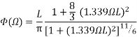
(2) Values of Ā must be determined according to the following formula:

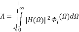
Where:

H(Ω) = the frequency response function, determined by dynamic analysis, that relates the loads in the aircraft structure to the atmospheric turbulence; and

Φ_I(Ω) = normalised power spectral density of atmospheric turbulence given by:

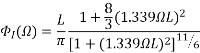
Where:

Ω  = reduced frequency, rad/ft; and

L   = scale of turbulence = 2,500 ft.

(3) The limit turbulence intensities, U_σ, in m/s (ft/s) true airspeed required for compliance with this paragraph are:

(i) At aeroplane speeds between V_B and V_C:

Where:

U_σref is the reference turbulence intensity that varies linearly with altitude from 27.43 m/s (90 ft/s) (TAS) at sea level to 24.08 m/s (79 ft/s) (TAS) at 7315 m (24000 ft) and is then constant at 24.08 m/s (79 ft/s) (TAS) up to the altitude of 18288 m (60000 ft); and

F_g is the flight profile alleviation factor defined in subparagraph (a)(6) of this paragraph;

(ii) At speed V_D: U_σ is equal to 1/2 the values obtained under subparagraph (3)(i) of this paragraph.

(iii) At speeds between V_C and V_D: Uσ is equal to a value obtained by linear interpolation.

(iv) At all speeds both positive and negative incremental loads due to continuous turbulence must be considered.

(4) When an automatic system affecting the dynamic response of the aeroplane is included in the analysis, the effects of system non-linearities on loads at the limit load level must be taken into account in a realistic or conservative manner.

(5) If necessary for the assessment of loads on aeroplanes with significant non-linearities, it must be assumed that the turbulence field has a root-mean-square velocity equal to 40 percent of the U_σ values specified in subparagraph (3). The value of limit load is that load with the same probability of exceedance in the turbulence field as ĀUσ of the same load quantity in a linear approximated model.

(c) Supplementary gust conditions for wing mounted engines. For aeroplanes equipped with wing mounted engines, the engine mounts, pylons, and wing supporting structure must be designed for the maximum response at the nacelle centre of gravity derived from the following dynamic gust conditions applied to the aeroplane:

(1) A discrete gust determined in accordance with CS 25.341(a) at each angle normal to the flight path, and separately,

(2) A pair of discrete gusts, one vertical and one lateral. The length of each of these gusts must be independently tuned to the maximum response in accordance with CS 25.341(a). The penetration of the aeroplane in the combined gust field and the phasing of the vertical and lateral component gusts must be established to develop the maximum response to the gust pair. In the absence of a more rational analysis, the following formula must be used for each of the maximum engine loads in all six degrees of freedom:

Where:

P_L   = limit load;

P_L-1g = steady 1-g load for the condition;

L_V   = peak incremental response load due to a vertical gust according to CS 25.341(a); and

L_L   = peak incremental response load due to a lateral gust according to CS 25.341(a).

[Amdt 25/1]

[Amdt 25/12]

AMC 25.341  Gust and Continuous Turbulence Design Criteria (Acceptable Means of Compliance)

ED Decision 2019/013/R

1. PURPOSE. This AMC sets forth an acceptable means of compliance with the provisions of CS-25 dealing with discrete gust and continuous turbulence dynamic loads. 

2. RELATED CERTIFICATION SPECIFICATIONS. The contents of this AMC are considered by the Agency in determining compliance with the discrete gust and continuous turbulence criteria defined in CS 25.341. Related paragraphs are:

CS 25.343  Design fuel and oil loads

CS 25.345  High lift devices

CS 25.349  Rolling conditions

CS 25.371  Gyroscopic loads

CS 25.373  Speed control devices

CS 25.391  Control surface loads

CS 25.427  Unsymmetrical loads

CS 25 445  Auxiliary aerodynamic surfaces

CS 25.571  Damage-tolerance and fatigue evaluation of structure

Reference should also be made to the following CS paragraphs: CS 25.301, CS 25.302, CS 25.303, CS 25.305, CS 25.321, CS 25.335, CS 25.1517.

3. OVERVIEW. This AMC addresses both discrete gust and continuous turbulence (or continuous gust) requirements of CS-25. It provides some of the acceptable methods of modelling aeroplanes, aeroplane components, and configurations, and the validation of those modelling methods for the purpose of determining the response of the aeroplane to encounters with gusts.

How the various aeroplane modelling parameters are treated in the dynamic analysis can have a large influence on design load levels. The basic elements to be modelled in the analysis are the elastic, inertial, aerodynamic and control system characteristics of the complete, coupled aeroplane (Figure 1). The degree of sophistication and detail required in the modelling depends on the complexity of the aeroplane and its systems.

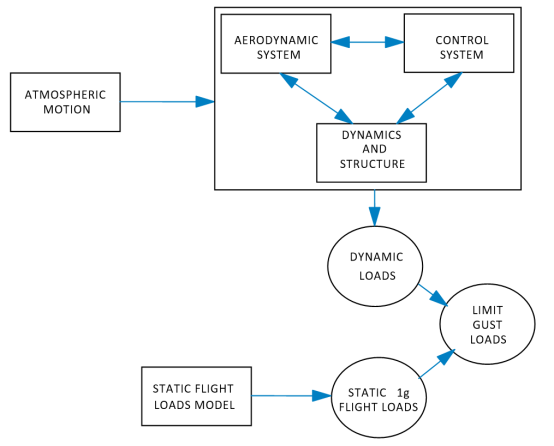
Figure 1 Basic Elements of the Gust Response Analysis

Design loads for encounters with gusts are a combination of the steady level 1-g flight loads, and the gust incremental loads including the dynamic response of the aeroplane. The steady 1-g flight loads can be realistically defined by the basic external parameters such as speed, altitude, weight and fuel load. They can be determined using static aeroelastic methods.

The gust incremental loads result from the interaction of atmospheric turbulence and aeroplane rigid body and elastic motions. They may be calculated using linear analysis methods when the aeroplane and its flight control systems are reasonably or conservatively approximated by linear analysis models.

Non-linear solution methods are necessary for aeroplane and flight control systems that are not reasonably or conservatively represented by linear analysis models. Non-linear features generally raise the level of complexity, particularly for the continuous turbulence analysis, because they often require that the solutions be carried out in the time domain. 

The modelling parameters discussed in the following paragraphs include:

—             Design conditions and associated steady, level 1-g flight conditions.

—             The discrete and continuous gust models of atmospheric turbulence.

—             Detailed representation of the aeroplane system including structural dynamics, aerodynamics, and control system modelling.

—             Solution of the equations of motion and the extraction of response loads.

—             Considerations for non-linear aeroplane systems.

—             Analytical model validation techniques.

4. DESIGN CONDITIONS.

 a. General. Analyses should be conducted to determine gust response loads for the aeroplane throughout its design envelope, where the design envelope is taken to include, for example, all appropriate combinations of aeroplane configuration, weight, centre of gravity, payload, fuel load, thrust, speed, and altitude.

 b. Steady Level 1-g Flight Loads.  The total design load is made up of static and dynamic load components. In calculating the static component, the aeroplane is assumed to be in trimmed steady level flight, either as the initial condition for the discrete gust evaluation or as the mean flight condition for the continuous turbulence evaluation. Static aeroelastic effects should be taken into account if significant.

 To ensure that the maximum total load on each part of the aeroplane is obtained, the associated steady-state conditions should be chosen in such a way as to reasonably envelope the range of possible steady-state conditions that could be achieved in that flight condition. Typically, this would include consideration of effects such as speed brakes, power settings between zero thrust and the maximum for the flight condition, etc.

c. Dynamic Response Loads.  The incremental loads from the dynamic gust solution are superimposed on the associated steady level flight 1-g loads. Load responses in both positive and negative senses should be assumed in calculating total gust response loads.  Generally the effects of speed brakes, flaps, or other drag or high lift devices, while they should be included in the steady-state condition, may be neglected in the calculation of incremental loads.

d. Damage Tolerance Conditions. Limit gust loads, treated as ultimate, need to be developed for the structural failure conditions considered under CS 25.571(b). Generally, for redundant structures, significant changes in stiffness or geometry do not occur for the types of damage under consideration. As a result, the limit gust load values obtained for the undamaged aircraft may be used and applied to the failed structure. However, when structural failures of the types considered under CS 25.571(b) cause significant changes in stiffness or geometry, or both, these changes should be taken into account when calculating limit gust loads for the damaged structure.

5. GUST MODEL CONSIDERATIONS.

a. General. The gust criteria presented in CS 25.341 consist of two models of atmospheric turbulence, a discrete model and a continuous turbulence model. It is beyond the scope of this AMC to review the historical development of these models and their associated parameters. This AMC focuses on the application of those gust criteria to establish design limit loads. The discrete gust model is used to represent single discrete extreme turbulence events. The continuous turbulence model represents longer duration turbulence encounters which excite lightly damped modes. Dynamic loads for both atmospheric models must be considered in the structural design of the aeroplane.

b. Discrete Gust Model

(1) Atmosphere. The atmosphere is assumed to be one dimensional with the gust velocity acting normal (either vertically or laterally) to the direction of aeroplane travel. The one-dimensional assumption constrains the instantaneous vertical or lateral gust velocities to be the same at all points in planes normal to the direction of aeroplane travel. Design level discrete gusts are assumed to have 1-cosine velocity profiles. The maximum velocity for a discrete gust is calculated using a reference gust velocity, U_ref, a flight profile alleviation factor, Fg, and an expression which modifies the maximum velocity as a function of the gust gradient distance, H. These parameters are discussed further below.

(A) Reference Gust Velocity, U_ref  - Derived effective gust velocities representing gusts occurring once in 70,000 flight hours are the basis for design gust velocities. These reference velocities are specified as a function of altitude in CS 25.341(a)(5) and are given in terms of feet per second equivalent airspeed for a gust gradient distance, H, of 107 m (350 ft).

(B) Flight Profile Alleviation Factor, F_g - The reference gust velocity, Uref , is a measure of turbulence intensity as a function of altitude. In defining the value of Uref at each altitude, it is assumed that the aircraft is flown 100% of the time at that altitude. The factor F_g is then applied to account for the expected service experience in terms of the probability of the aeroplane flying at any given altitude within its certification altitude range. Fg is a minimum value at sea level, linearly increasing to 1.0 at the certified maximum altitude. The expression for Fg is given in CS 25.341(a)(6).

(C) Gust Gradient Distance, H - The gust gradient distance is that distance over which the gust velocity increases to a maximum value. Its value is specified as ranging from 9.1 to 107 m (30 to 350 ft). (It should be noted that if 12.5 times the mean geometric chord of the aeroplane’s wing exceeds 350 ft, consideration should be given to covering increased maximum gust gradient distances.)

(D) Design Gust Velocity, U_ds - Maximum velocities for design gusts are proportional to the sixth root of the gust gradient distance, H. The maximum gust velocity for a given gust is then defined as:

The maximum design gust velocity envelope, Uds, and example design gust velocity profiles are illustrated in Figure 2.

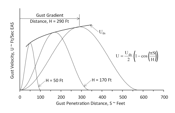
Figure-2  Typical (1-cosine) Design Gust Velocity Profiles

(2) Discrete Gust Response. The solution for discrete gust response time histories can be achieved by a number of techniques. These include the explicit integration of the aeroplane equations of motion in the time domain, and frequency domain solutions utilising Fourier transform techniques. These are discussed further in Paragraph 7.0 of this AMC.

Maximum incremental loads, P_Ii, are identified by the peak values selected from time histories arising from a series of separate, 1-cosine shaped gusts having gradient distances ranging from 9.1 to 107 m (30 to 350 ft). Input gust profiles should cover this gradient distance range in sufficiently small increments to determine peak loads and responses. Historically 10 to 20 gradient distances have been found to be acceptable. Both positive and negative gust velocities should be assumed in calculating total gust response loads. It should be noted that in some cases, the peak incremental loads can occur well after the prescribed gust velocity has returned to zero.  In such cases, the gust response calculation should be run for sufficient additional time to ensure that the critical incremental loads are achieved.

The design limit load, P_Li , corresponding to the maximum incremental load, P_Ii for a given load quantity is then defined as:

Where P_(1-g)i is the 1-g steady load for the load quantity under consideration. The set of time correlated design loads, P_Lj , corresponding to the peak value of the load quantity, P_Li, are calculated for the same instant in time using the expression:

Note that in the case of a non-linear aircraft, maximum positive incremental loads may differ from maximum negative incremental loads.

 When calculating stresses which depend on a combination of external loads it may be necessary to consider time correlated load sets at time instants other than those which result in peaks for individual external load quantities.

(3) Round-The-Clock Gust. When the effect of combined vertical and lateral gusts on aeroplane components is significant, then round-the-clock analysis should be conducted on these components and supporting structures. The vertical and lateral components of the gust are assumed to have the same gust gradient distance, H and to start at the same time. Components that should be considered include horizontal tail surfaces having appreciable dihedral or anhedral (i.e., greater than 10º), or components supported by other lifting surfaces, for example T-tails, outboard fins and winglets. Whilst the round-the-clock load assessment may be limited to just the components under consideration, the loads themselves should be calculated from a whole aeroplane dynamic analysis.

The round-the-clock gust model assumes that discrete gusts may act at any angle normal to the flight path of the aeroplane. Lateral and vertical gust components are correlated since the round-the-clock gust is a single discrete event. For a linear aeroplane system, the loads due to a gust applied from a direction intermediate to the vertical and lateral directions - the round-the-clock gust loads - can be obtained using a linear combination of the load time histories induced from pure vertical and pure lateral gusts. The resultant incremental design value for a particular load of interest is obtained by determining the round-the-clock gust angle and gust length giving the largest (tuned) response value for that load. The design limit load is then obtained using the expression for P_L given above in paragraph 5(b)(2).

(4) Supplementary Gust Conditions for Wing Mounted Engines.

(A) Atmosphere - For aircraft equipped with wing mounted engines, CS 25.341(c) requires that engine mounts, pylons and wing supporting structure be designed to meet a round-the-clock discrete gust requirement and a multi-axis discrete gust requirement.

The model of the atmosphere and the method for calculating response loads for the round-the-clock gust requirement is the same as that described in Paragraph 5(b)(3) of this AMC.

For the multi-axis gust requirement, the model of the atmosphere consists of two independent discrete gust components, one vertical and one lateral, having amplitudes such that the overall probability of the combined gust pair is the same as that of a single discrete gust as defined by CS 25.341(a) as described in Paragraph 5(b)(1) of this AMC. To achieve this equal-probability condition, in addition to the reductions in gust amplitudes that would be applicable if the input were a multi-axis Gaussian process, a further factor of 0.85 is incorporated into the gust amplitudes to account for non-Gaussian properties of severe discrete gusts. This factor was derived from severe gust data obtained by a research aircraft specially instrumented to measure vertical and lateral gust components. This information is contained in Stirling Dynamics Laboratories Report No SDL –571-TR-2 dated May 1999.

(B)  Multi-Axis Gust Response - For a particular aircraft flight condition, the calculation of a specific response load requires that the amplitudes, and the time phasing, of the two gust components be chosen, subject to the condition on overall probability specified in (A) above, such that the resulting combined load is maximised. For loads calculated using a linear aircraft model, the response load may be based upon the separately tuned vertical and lateral discrete gust responses for that load, each calculated as described in Paragraph 5(b)(2) of this AMC. In general, the vertical and lateral tuned gust lengths and the times to maximum response (measured from the onset of each gust) will not be the same.

Denote the independently tuned vertical and lateral incremental responses for a particular aircraft flight condition and load quantity i by L_Vi and L_Li, respectively. The associated multi-axis gust input is obtained by multiplying the amplitudes of the independently-tuned vertical and lateral discrete gusts, obtained as described in the previous paragraph, by 0.85*L_Vi/√ (L_Vi²+L_Li²) and 0.85*L_Li/√ (L_Vi²+L_Li²) respectively. The time-phasing of the two scaled gust components is such that their associated peak loads occur at the same instant.

The combined incremental response load is given by:

and the design limit load, P_Li, corresponding to the maximum incremental load, P_Ii, for the given load quantity is then given by:

where P_(1-g)i is the 1-g steady load for the load quantity under consideration.

The incremental, time correlated loads corresponding to the specific flight condition under consideration are obtained from the independently-tuned vertical and lateral gust inputs for load quantity i.  The vertical and lateral gust amplitudes are factored by 0.85*L_Vi/√ (L_Vi²+L_Li²) and 0.85*L_Li/√(L_Vi²+L_Li²) respectively. Loads L_Vj and L_Lj resulting from these reduced vertical and lateral gust inputs, at the time when the amplitude of load quantity i is at a maximum value, are added to yield the multi-axis incremental time-correlated value P_Ij for load quantity j.

The set of time correlated design loads, P_Lj , corresponding to the peak value of the load quantity, P_Li, are obtained using the expression:

Note that with significant non-linearities, maximum positive incremental loads may differ from maximum negative incremental loads.

c. Continuous Turbulence Model.

(1) Atmosphere. The atmosphere for the determination of continuous gust responses is assumed to be one dimensional with the gust velocity acting normal (either vertically or laterally) to the direction of aeroplane travel. The one-dimensional assumption constrains the instantaneous vertical or lateral gust velocities to be the same at all points in planes normal to the direction of aeroplane travel.

The random atmosphere is assumed to have a Gaussian distribution of gust velocity intensities and a Von Kármán power spectral density with a scale of turbulence, L, equal to 2500 feet. The expression for the Von Kármán spectrum for unit, root-mean-square (RMS) gust intensity, Φ_I(Ω), is given below. In this expression Ω = ω/V, where ω is the circular frequency in radians per second, and V is the aeroplane velocity in feet per second true airspeed.

The Von Kármán power spectrum for unit RMS gust intensity is illustrated in Figure 3.

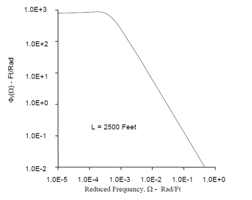
Figure-3  The Von Kármán Power Spectral Density Function, ΦI(Ω)

 The design gust velocity, Uσ, applied in the analysis is given by the product of the reference gust velocity, Uσref , and the profile alleviation factor, Fg, as follows:

where values for Uσref , are specified in CS 25.341(b)(3) in meters per second (feet per second) true airspeed and Fg is defined in CS 25.341(a)(6). The value of Fg is based on aeroplane design parameters and is a minimum value at sea level, linearly increasing to 1.0 at the certified maximum design altitude. It is identical to that used in the discrete gust analysis.

As for the discrete gust analysis, the reference continuous turbulence gust intensity, Uσref, defines the design value of the associated gust field at each altitude. In defining the value of Uσref at each altitude, it is assumed that the aeroplane is flown 100% of the time at that altitude. The factor Fg is then applied to account for the probability of the aeroplane flying at any given altitude during its service lifetime.

It should be noted that the reference gust velocity is comprised of two components, a root-mean-square (RMS) gust intensity and a peak to RMS ratio. The separation of these components is not defined and is not required for the linear aeroplane analysis. Guidance is provided in Paragraph 8.d. of this AMC for generating a RMS gust intensity for a non-linear simulation.

(2) Continuous Turbulence Response. For linear aeroplane systems, the solution for the response to continuous turbulence may be performed entirely in the frequency domain, using the RMS response. is defined in CS 25.341(b)(2) and is repeated here in modified notation for load quantity i, where:

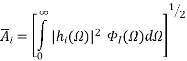
or

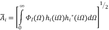
In the above expression Φ_I(Ω) is the input Von Kármán power spectrum of the turbulence and is defined in Paragraph 5.c.(1) of this AMC, h_i(iΩ) is the transfer function relating the output load quantity, i, to a unit, harmonically oscillating, one-dimensional gust field, and the asterisk superscript denotes the complex conjugate. When evaluating Ā_i, the integration should be continued until a converged value is achieved since, realistically, the integration to infinity may be impractical. The design limit load, P_Li, is then defined as:

where U_σ is defined in Paragraph 5.c.(1) of this AMC, and P_(1-g)i is the 1-g steady state value for the load quantity, i, under consideration. As indicated by the formula, both positive and negative load responses should be considered when calculating limit loads.

Correlated (or equiprobable) loads can be developed using cross-correlation coefficients, ρ_ij, computed as follows:

where, ‘real[...]’ denotes the real part of the complex function contained within the brackets. In this equation, the lowercase subscripts, i and j, denote the responses being correlated. A set of design loads, P_Lj, correlated to the design limit load P_Li, are then calculated as follows:

The correlated load sets calculated in the foregoing manner provide balanced load distributions corresponding to the maximum value of the response for each external load quantity, i, calculated.

When calculating stresses, the foregoing load distributions may not yield critical design values because critical stress values may depend on a combination of external loads. In these cases, a more general application of the correlation coefficient method is required. For example, when the value of stress depends on two externally applied loads, such as torsion and shear, the equiprobable relationship between the two parameters forms an ellipse as illustrated in Figure 4.

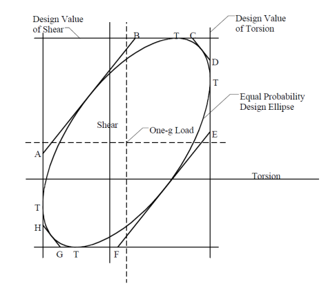
Figure-4  Equal Probability Design Ellipse

In this figure, the points of tangency, T, correspond to the expressions for correlated load pairs given by the foregoing expressions. A practical additional set of equiprobable load pairs that should be considered to establish critical design stresses are given by the points of tangency to the ellipse by lines AB, CD, EF and GH. These additional load pairs are given by the following expressions (where i = torsion and j = shear):

For tangents to lines AB and EF

and

For tangents to lines CD and GH

and

All correlated or equiprobable loads developed using correlation coefficients will provide balanced load distributions.

A more comprehensive approach for calculating critical design stresses that depend on a combination of external load quantities is to evaluate directly the transfer function for the stress quantity of interest from which can be calculated the gust response function, the value for RMS response, Ā, and the design stress values P(1-g) ± U_σ Ā.

6. AEROPLANE MODELLING CONSIDERATIONS

a. General. The procedures presented in this paragraph generally apply for aeroplanes having aerodynamic and structural properties and flight control systems that may be reasonably or conservatively approximated using linear analysis methods for calculating limit load. Additional guidance material is presented in Paragraph 8 of this AMC for aeroplanes having properties and/or systems not reasonably or conservatively approximated by linear analysis methods.

b. Structural Dynamic Model. The model should include both rigid body and flexible aeroplane degrees of freedom. If a modal approach is used, the structural dynamic model should include a sufficient number of flexible aeroplane modes to ensure both convergence of the modal superposition procedure and that responses from high frequency excitations are properly represented.

Most forms of structural modelling can be classified into two main categories: (1) the so-called “stick model” characterised by beams with lumped masses distributed along their lengths, and (2) finite element models in which all major structural components (frames, ribs, stringers, skins) are represented with mass properties defined at grid points. Regardless of the approach taken for the structural modelling, a minimum acceptable level of sophistication, consistent with configuration complexity, is necessary to represent satisfactorily the critical modes of deformation of the primary structure and control surfaces. Results from the models should be compared to test data as outlined in Paragraph 9.b. of this AMC in order to validate the accuracy of the model.

c. Structural Damping.  Structural dynamic models may include damping properties in addition to representations of mass and stiffness distributions. In the absence of better information it will normally be acceptable to assume 0.03 (i.e. 1.5% equivalent critical viscous damping) for all flexible modes. Structural damping may be increased over the 0.03 value to be consistent with the high structural response levels caused by extreme gust intensity, provided justification is given.

d. Gust and Motion Response Aerodynamic Modelling. Aerodynamic forces included in the analysis are produced by both the gust velocity directly, and by the aeroplane response.

Aerodynamic modelling for dynamic gust response analyses requires the use of unsteady two-dimensional or three-dimensional panel theory methods for incompressible or compressible flow. The choice of the appropriate technique depends on the complexity of the aerodynamic configuration, the dynamic motion of the surfaces under investigation and the flight speed envelope of the aeroplane. Generally, three-dimensional panel methods achieve better modelling of the aerodynamic interference between lifting surfaces. The model should have a sufficient number of aerodynamic degrees of freedom to properly represent the steady and unsteady aerodynamic distributions under consideration.

The build-up of unsteady aerodynamic forces should be represented. In two-dimensional unsteady analysis this may be achieved in either the frequency domain or the time domain through the application of oscillatory or indicial lift functions, respectively. Where three-dimensional panel aerodynamic theories are to be applied in the time domain (e.g. for non-linear gust solutions), an approach such as the ‘rational function approximation’ method may be employed to transform frequency domain aerodynamics into the time domain.

Oscillatory lift functions due to gust velocity or aeroplane response depend on the reduced frequency parameter, k. The maximum reduced frequency used in the generation of the unsteady aerodynamics should include the highest frequency of gust excitation and the highest structural frequency under consideration. Time lags representing the effect of the gradual penetration of the gust field by the aeroplane should also be accounted for in the build-up of lift due to gust velocity.

The aerodynamic modelling should be supported by tests or previous experience as indicated in Paragraph 9.d. of this AMC. Primary lifting and control surface distributed aerodynamic data are commonly adjusted by weighting factors in the dynamic gust response analyses. The weighting factors for steady flow (k = 0) may be obtained by comparing wind tunnel test results with theoretical data. The correction of the aerodynamic forces should also ensure that the rigid body motion of the aeroplane is accurately represented in order to provide satisfactory short period and Dutch roll frequencies and damping ratios. Corrections to primary surface aerodynamic loading due to control surface deflection should be considered.  Special attention should also be given to control surface hinge moments and to fuselage and nacelle aerodynamics because viscous and other effects may require more extensive adjustments to the theoretical coefficients. Aerodynamic gust forces should reflect weighting factor adjustments performed on the steady or unsteady motion response aerodynamics.

e. Gyroscopic Loads. As specified in CS 25.371, the structure supporting the engines and the auxiliary power units should be designed for the gyroscopic loads induced by both discrete gusts and continuous turbulence. The gyroscopic loads for turbopropellers and turbofans may be calculated as an integral part of the solution process by including the gyroscopic terms in the equations of motion or the gyroscopic loads can be superimposed after the solution of the equations of motion. Propeller and fan gyroscopic coupling forces (due to rotational direction) between symmetric and antisymmetric modes need not be taken into account if the coupling forces are shown to be negligible.

The gyroscopic loads used in this analysis should be determined with the engine or auxiliary power units at maximum continuous rpm. The mass polar moment of inertia used in calculating gyroscopic inertia terms should include the mass polar moments of inertia of all significant rotating parts taking into account their respective rotational gearing ratios and directions of rotation.

f. Control Systems. Gust analyses of the basic configuration should include simulation of any control system for which interaction may exist with the rigid body response, structural dynamic response or external loads. If possible, these control systems should be uncoupled such that the systems which affect “symmetric flight” are included in the vertical gust analysis and those which affect “antisymmetric flight” are included in the lateral gust analysis.

The control systems considered should include all relevant modes of operation. Failure conditions should also be analysed for any control system which influences the design loads in accordance with CS 25.302 and Appendix K.

The control systems included in the gust analysis may be assumed to be linear if the impact of the non-linearity is negligible, or if it can be shown by analysis on a similar aeroplane/control system that a linear control law representation is conservative. If the control system is significantly non-linear, and a conservative linear approximation to the control system cannot be developed, then the effect of the control system on the aeroplane responses should be evaluated in accordance with Paragraph 8. of this AMC.

g. Stability. Solutions of the equations of motion for either discrete gusts or continuous turbulence require the dynamic model be stable. This applies for all modes, except possibly for very low frequency modes which do not affect load responses, such as the phugoid mode. (Note that the short period and Dutch roll modes do affect load responses). A stability check should be performed for the dynamic model using conventional stability criteria appropriate for the linear or non-linear system in question, and adjustments should be made to the dynamic model, as required, to achieve appropriate frequency and damping characteristics.

 If control system models are to be included in the gust analysis it is advisable to check that the following characteristics are acceptable and are representative of the aeroplane:

—             static margin of the unaugmented aeroplane

—             dynamic stability of the unaugmented aeroplane

—             the static aeroelastic effectiveness of all control surfaces utilised by any feed-back control system

—             gain and phase margins of any feedback control system coupled with the aeroplane rigid body and flexible modes

—             the aeroelastic flutter and divergence margins of the unaugmented aeroplane, and also for any feedback control system coupled with the aeroplane.

7. DYNAMIC LOADS

a. General. This paragraph describes methods for formulating and solving the aeroplane equations of motion and extracting dynamic loads from the aeroplane response. The aeroplane equations of motion are solved in either physical or modal co-ordinates and include all terms important in the loads calculation including stiffness, damping, mass, and aerodynamic forces due to both aeroplane motions and gust excitation. Generally the aircraft equations are solved in modal co-ordinates. For the purposes of describing the solution of these equations in the remainder of this AMC, modal co-ordinates will be assumed. A sufficient number of modal co-ordinates should be included to ensure that the loads extracted provide converged values.

b.  Solution of the Equations of Motion. Solution of the equations of motion can be achieved through a number of techniques. For the continuous turbulence analysis, the equations of motion are generally solved in the frequency domain. Transfer functions which relate the output response quantity to an input harmonically oscillating gust field are generated and these transfer functions are used (in Paragraph 5.c. of this AMC) to generate the RMS value of the output response quantity.

There are two primary approaches used to generate the output time histories for the discrete gust analysis; (1) by explicit integration of the aeroplane equations of motion in the time domain, and (2) by frequency domain solutions which can utilise Fourier transform techniques.

c. Extraction of Loads and Responses.  The output quantities that may be extracted from a gust response analysis include displacements, velocities and accelerations at structural locations; load quantities such as shears, bending moments and torques on structural components; and stresses and shear flows in structural components. The calculation of the physical responses is given by a modal superposition of the displacements, velocities and accelerations of the rigid and elastic modes of vibration of the aeroplane structure. The number of modes carried in the summation should be sufficient to ensure converged results.

A variety of methods may be used to obtain physical structural loads from a solution of the modal equations of motion governing gust response. These include the Mode Displacement method, the Mode Acceleration method, and the Force Summation method. All three methods are capable of providing a balanced set of aeroplane loads. If an infinite number of modes can be considered in the analysis, the three will lead to essentially identical results.

The Mode Displacement method is the simplest. In this method, total dynamic loads are calculated from the structural deformations produced by the gust using modal superposition. Specifically, the contribution of a given mode is equal to the product of the load associated with the normalised deformed shape of that mode and the value of the displacement response given by the associated modal co-ordinate. For converged results, the Mode Displacement method may need a significantly larger number of modal co-ordinates than the other two methods. 

In the Mode Acceleration method, the dynamic load response is composed of a static part and a dynamic part. The static part is determined by conventional static analysis (including rigid body “inertia relief”), with the externally applied gust loads treated as static loads. The dynamic part is computed by the superposition of appropriate modal quantities, and is a function of the number of modes carried in the solution. The quantities to be superimposed involve both motion response forces and acceleration responses (thus giving this method its name). Since the static part is determined completely and independently of the number of normal modes carried, adequate accuracy may be achieved with fewer modes than would be needed in the Mode Displacement method.

The Force Summation method is the most laborious and the most intuitive. In this method, physical displacements, velocities and accelerations are first computed by superposition of the modal responses. These are then used to determine the physical inertia forces and other motion dependent forces. Finally, these forces are added to the externally applied forces to give the total dynamic loads acting on the structure.

If balanced aeroplane load distributions are needed from the discrete gust analysis, they may be determined using time correlated solution results.  Similarly, as explained in Paragraph 5.c of this AMC, if balanced aeroplane load distributions are needed from the continuous turbulence analysis, they may be determined from equiprobable solution results obtained using cross-correlation coefficients.

8. NONLINEAR CONSIDERATIONS

a. General. Any structural, aerodynamic or automatic control system characteristic which may cause aeroplane response to discrete gusts or continuous turbulence to become non-linear with respect to intensity or shape should be represented realistically or conservatively in the calculation of loads. While many minor non-linearities are amenable to a conservative linear solution, the effect of major non-linearities cannot usually be quantified without explicit calculation.

The effect of non-linearities should be investigated above limit conditions to assure that the system presents no anomaly compared to behaviour below limit conditions, in accordance with Appendix K, K25.2(b)(2).

b. Structural and Aerodynamic Non-linearity. A linear elastic structural model, and a linear (unstalled) aerodynamic model are normally recommended as conservative and acceptable for the unaugmented aeroplane elements of a loads calculation. Aerodynamic models may be refined to take account of minor non-linear variation of aerodynamic distributions, due to local separation etc., through simple linear piecewise solution. Local or complete stall of a lifting surface would constitute a major non-linearity and should not be represented without account being taken of the influence of rate of change of incidence, i.e., the so-called ‘dynamic stall’ in which the range of linear incremental aerodynamics may extend significantly beyond the static stall incidence.

c. Automatic Control System Non-linearity. Automatic flight control systems, autopilots, stability control systems and load alleviation systems often constitute the primary source of non-linear response. For example,

—             non-proportional feedback gains

—             rate and amplitude limiters

—             changes in the control laws, or control law switching

—             hysteresis

—             use of one-sided aerodynamic controls such as spoilers

—             hinge moment performance and saturation of aerodynamic control actuators

The resulting influences on response will be aeroplane design dependent, and the manner in which they are to be considered will normally have to be assessed for each design.

Minor influences such as occasional clipping of response due to rate or amplitude limitations, where it is symmetric about the stabilised 1-g condition, can often be represented through quasi-linear modelling techniques such as describing functions or use of a linear equivalent gain.

Major, and unsymmetrical influences such as application of spoilers for load alleviation, normally require explicit simulation, and therefore adoption of an appropriate solution based in the time domain.

The influence of non-linearities on one load quantity often runs contrary to the influence on other load quantities. For example, an aileron used for load alleviation may simultaneously relieve wing bending moment whilst increasing wing torsion. Since it may not be possible to represent such features conservatively with a single aeroplane model, it may be conservatively acceptable to consider loads computed for two (possibly linear) representations which bound the realistic condition. Another example of this approach would be separate representation of continuous turbulence response for the two control law states to cover a situation where the aeroplane may occasionally switch from one state to another.

d. Non-linear Solution Methodology.  Where explicit simulation of non-linearities is required, the loads response may be calculated through time domain integration of the equations of motion.

For the tuned discrete gust conditions of CS 25.341(a), limit loads should be identified by peak values in the non-linear time domain simulation response of the aeroplane model excited by the discrete gust model described in Paragraph 5.b. of this AMC.

For time domain solution of the continuous turbulence conditions of CS 25.341(b), a variety of approaches may be taken for the specification of the turbulence input time history and the mechanism for identifying limit loads from the resulting responses.

It will normally be necessary to justify that the selected approach provides an equivalent level of safety as a conventional linear analysis and is appropriate to handle the types of non-linearity on the aircraft. This should include verification that the approach provides adequate statistical significance in the loads results.

A methodology based upon stochastic simulation has been found to be acceptable for load alleviation and flight control system non-linearities. In this simulation, the input is a long, Gaussian, pseudo-random turbulence stream conforming to a Von Kármán spectrum with a root-mean-square (RMS) amplitude of 0.4 times U_σ (defined in Paragraph 5.c (1) of this AMC). The value of limit load is that load with the same probability of exceedance as Ā U_σ of the same load quantity in a linear model. This is illustrated graphically in Figure 5. When using an analysis of this type, exceedance curves should be constructed using incremental load values up to, or just beyond the limit load value.

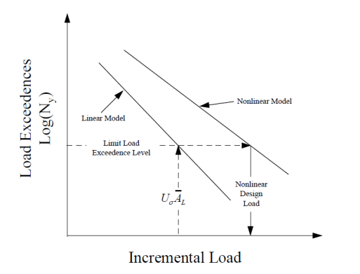
Figure-5  Establishing Limit Load for a Non-linear Aeroplane

The non-linear simulation may also be performed in the frequency domain if the frequency domain method is shown to produce conservative results. Frequency domain methods include, but are not limited to, Matched Filter Theory and Equivalent Linearisation.

9. ANALYTICAL MODEL VALIDATION

a. General. The intent of analytical model validation is to establish that the analytical model is adequate for the prediction of gust response loads. The following paragraphs discuss acceptable but not the only methods of validating the analytical model. In general, it is not intended that specific testing be required to validate the dynamic gust loads model.

b. Structural Dynamic Model Validation. The methods and test data used to validate the flutter analysis models presented in AMC 25.629 should also be applied to validate the gust analysis models. These procedures are addressed in AMC 25.629.

c. Damping Model Validation. In the absence of better information it will normally be acceptable to assume 0.03 (i.e. 1.5% equivalent critical viscous damping) for all flexible modes. Structural damping may be increased over the 0.03 value to be consistent with the high structural response levels caused by extreme gust intensity, provided justification is given.

d. Aerodynamic Model Validation. Aerodynamic modelling parameters fall into two categories:

(i) steady or quasi-steady aerodynamics governing static aeroelastic and flight dynamic airload distributions

(ii) unsteady aerodynamics which interact with the flexible modes of the aeroplane.

Flight stability aerodynamic distributions and derivatives may be validated by wind tunnel tests, detailed aerodynamic modelling methods (such as CFD) or flight test data. If detailed analysis or testing reveals that flight dynamic characteristics of the aeroplane differ significantly from those to which the gust response model have been matched, then the implications on gust loads should be investigated.

The analytical and experimental methods presented in AMC 25.629 for flutter analyses provide acceptable means for establishing reliable unsteady aerodynamic characteristics both for motion response and gust excitation aerodynamic force distributions. The aeroelastic implications on aeroplane flight dynamic stability should also be assessed.

e. Control System Validation. If the aeroplane mathematical model used for gust analysis contains a representation of any feedback control system, then this segment of the model should be validated. The level of validation that should be performed depends on the complexity of the system and the particular aeroplane response parameter being controlled. Systems which control elastic modes of the aeroplane may require more validation than those which control the aeroplane rigid body response. Validation of elements of the control system (sensors, actuators, anti-aliasing filters, control laws, etc.) which have a minimal effect on the output load and response quantities under consideration can be neglected.

It will normally be more convenient to substantiate elements of the control system independently, i.e. open loop, before undertaking the validation of the closed loop system.

(1) System Rig or Aeroplane Ground Testing. Response of the system to artificial stimuli can be measured to verify the following:

—             The transfer functions of the sensors and any pre-control system anti-aliasing or other filtering.

—             The sampling delays of acquiring data into the control system.

—             The behaviour of the control law itself.

—             Any control system output delay and filter transfer function.

—             The transfer functions of the actuators, and any features of actuation system performance characteristics that may influence the actuator response to the maximum demands that might arise in turbulence; e.g. maximum rate of deployment, actuator hinge moment capability, etc.

If this testing is performed, it is recommended that following any adaptation of the model to reflect this information, the complete feedback path be validated (open loop) against measurements taken from the rig or ground tests.

(2) Flight Testing. The functionality and performance of any feedback control system can also be validated by direct comparison of the analytical model and measurement for input stimuli. If this testing is performed, input stimuli should be selected such that they exercise the features of the control system and the interaction with the aeroplane that are significant in the use of the mathematical model for gust load analysis. These might include:

—             Aeroplane response to pitching and yawing manoeuvre demands.

—             Control system and aeroplane response to sudden artificially introduced demands such as pulses and steps.

—             Gain and phase margins determined using data acquired within the flutter test program. These gain and phase margins can be generated by passing known signals through the open loop system during flight test.

[Amdt No: 25/1]

[Amdt No: 25/23]

CS 25.343 Design fuel and oil loads

ED Decision 2005/006/R

(a) The disposable load combinations must include each fuel and oil load in the range from zero fuel and oil to the selected maximum fuel and oil load. A structural reserve fuel condition, not exceeding 45 minutes of fuel under operating conditions in CS 25.1001(f), may be selected.

(b) If a structural reserve fuel condition is selected, it must be used as the minimum fuel weight condition for showing compliance with the flight load requirements as prescribed in this Subpart. In addition –

(1) The structure must be designed for a condition of zero fuel and oil in the wing at limit loads corresponding to –

(i) A manoeuvring load factor of +2·25; and

(ii) The gust and turbulence conditions of CS 25.341, but assuming 85% of the gust velocities prescribed in CS 25.341(a)(4) and 85% of the turbulence intensities prescribed in CS 25.341(b)(3).

(2) Fatigue evaluation of the structure must account for any increase in operating stresses resulting from the design condition of sub-paragraph (b)(1) of this paragraph; and

(3) The flutter, deformation, and vibration requirements must also be met with zero fuel.

[Amdt 25/1]

CS 25.345 High lift devices

ED Decision 2016/010/R

(See AMC 25.345)

(a) If wing-flaps are to be used during take-off, approach, or landing, at the design flap speeds established for these stages of flight under CS 25.335(e) and with the wing-flaps in the corresponding positions, the aeroplane is assumed to be subjected to symmetrical manoeuvres and gusts. The resulting limit loads must correspond to the conditions determined as follows:

(1) Manoeuvring to a positive limit load factor of 2·0; and

(2) Positive and negative gusts of 7.62 m/sec (25 ft/sec) EAS acting normal to the flight path in level flight. Gust loads resulting on each part of the structure must be determined by rational analysis. The analysis must take into account the unsteady aerodynamic characteristics and rigid body motions of the aircraft. (See AMC 25.345(a).) The shape of the gust must be as described in CS 25.341(a)(2) except that –

U_ds  = 7.62 m/sec (25 ft/sec) EAS;

H    = 12.5 c; and

c     = mean geometric chord of the wing (metres (feet)).

(b) The aeroplane must be designed for the conditions prescribed in sub-paragraph (a) of this paragraph except that the aeroplane load factor need not exceed 1·0, taking into account, as separate conditions, the effects of –

(1) Propeller slipstream corresponding to maximum continuous power at the design flap speeds V_F, and with take-off power at not less than 1·4 times the stalling speed for the particular flap position and associated maximum weight; and

(2) A head-on gust of 7.62m/sec (25 fps) velocity (EAS).

(c) If flaps or other high lift devices are to be used in en-route conditions, and with flaps in the appropriate position at speeds up to the flap design speed chosen for these conditions, the aeroplane is assumed to be subjected to symmetrical manoeuvres and gusts within the range determined by –

(1) Manoeuvring to a positive limit load factor as prescribed in CS 25.337(b) ; and

(2) The vertical gust and turbulence conditions prescribed in CS 25.341. (See AMC 25.345(c).)

(d) The aeroplane must be designed for a manoeuvring load factor of 1.5 g at the maximum take-off weight with the wing-flaps and similar high lift devices in the landing configurations.

[Amdt 25/1]

[Amdt 25/18]

AMC 25.345(a) High lift devices (Gust conditions)

ED Decision 2003/2/RM

Compliance with CS 25.345(a) may be demonstrated by an analysis in which the solution of the vertical response equations is made by assuming the aircraft to be rigid. If desired, the analysis may take account of the effects of structural flexibility on a quasi-flexible basis (i.e. using aerodynamic derivatives and load distributions corresponding to the distorted structure under maximum gust load).

AMC 25.345(c) High lift devices (Procedure flight condition)

ED Decision 2003/2/RM

1  En-route conditions are flight segments other than take-off, approach and landing. As applied to the use of high lift devices the following flight phases are to be included in en-route conditions:

—             holding in designated areas outside the terminal area of the airport, and

—             flight with flaps extended from top of descent.

The following flight phases are not to be included in en-route conditions:

—             portion of the flight corresponding to standard arrival routes preceding the interception of the final approach path, and

—             holding at relatively low altitude close to the airport.

2 To apply CS 25.341(a) gust conditions to CS 25.345(c), the speeds V_FC and V_FD should be determined for the flap positions selected in en-route conditions.

These procedures should ensure proper speed margins for flap retraction in the case of severe turbulence when the aeroplane is in a low speed en-route holding configuration.

3 The manoeuvre of CS 25.345(c)(1) is to be considered as a balanced condition. (See CS 25.331(b) for definition.)

CS 25.349 Rolling conditions

ED Decision 2016/010/R

(See AMC 25.349)

The aeroplane must be designed for loads resulting from the rolling conditions specified in sub-paragraphs (a) and (b) of this paragraph. Unbalanced aerodynamic moments about the centre of gravity must be reacted in a rational or conservative manner, considering the principal masses furnishing the reacting inertia forces.

(a) Manoeuvring.  The following conditions, speeds, aileron deflections and cockpit roll control motions (except as the deflections and the motions may be limited by pilot effort) must be considered in combination with an aeroplane load factor of zero and of two-thirds of the positive manoeuvring factor used in design. For aeroplanes equipped with electronic flight controls, where the motion of the control surfaces does not bear a direct relationship to the motion of the cockpit control devices, these conditions must be considered in combination with an aeroplane load factor ranging from zero to two thirds of the positive manoeuvring factor used in design. In determining the required or resulting aileron deflections, the torsional flexibility of the wing must be considered in accordance with CS 25.301(b):

(1) Conditions corresponding to steady rolling velocities must be investigated. In addition, conditions corresponding to maximum angular acceleration must be investigated for aeroplanes with engines or other weight concentrations outboard of the fuselage, and for aeroplanes equipped with electronic flight controls, where the motion of the control surfaces does not bear a direct relationship to the motion of the cockpit control devices. For the angular acceleration conditions, zero rolling velocity may be assumed in the absence of a rational time history investigation of the manoeuvre.

(2) At V_A, a sudden deflection of the aileron to the stop is assumed.

(3) At V_C, the aileron deflection must be that required to produce a rate of roll not less than that obtained in sub-paragraph (a)(2) of this paragraph.

(4) At V_D, the aileron deflection must be that required to produce a rate of roll not less than one-third of that in sub-paragraph (a)(2) of this paragraph.

(5) For aeroplanes equipped with electronic flight controls, where the motion of the control surfaces does not bear a direct relationship to the motion of the cockpit control devices, in lieu of subparagraphs (a)(2), (a)(3), and (a)(4), the following apply:

(i) At V_A, movement of the cockpit roll control up to the limit is assumed. The position of the cockpit roll control must be maintained until a steady roll rate is achieved and then it must be returned suddenly to the neutral position.

(ii) At V_C, the cockpit roll control must be moved suddenly and maintained so as to achieve a roll rate not less than that obtained in subparagraph (a)(5)(i) of this paragraph. The return of cockpit control to neutral is initiated suddenly when steady roll rate is reached.

(iii) At V_D, the cockpit roll control must be moved suddenly and maintained so as to achieve a roll rate not less than one third of that obtained in subparagraph (a)(5)(i) of this paragraph.

  The conditions specified in this subparagraph must be investigated without any corrective yaw control action (pilot or system induced) to maximise sideslip, and, as a separate condition, with corrective yaw control action (pilot or system induced) to reduce sideslip as far as possible. The first condition (without any corrective yaw control action) may be considered as a failure condition under CS 25.302.

(See AMC 25.349(a))

(b) Unsymmetrical gusts. The aeroplane is assumed to be subjected to unsymmetrical vertical gusts in level flight. The resulting limit loads must be determined from either the wing maximum airload derived directly from CS 25.341(a), or the wing maximum airload derived indirectly from the vertical load factor calculated from CS 25.341(a). It must be assumed that 100 percent of the wing airload acts on one side of the aeroplane and 80 percent of the wing airload acts on the other side.

[Amdt 25/13]

[Amdt 25/18]

AMC 25.349(a) Rolling conditions

ED Decision 2013/010/R

The physical limitations of the aircraft from the cockpit roll control device to the control surface deflection, such as control stops position, maximum power and displacement rate of the servo controls, and control law limiters, may be taken into account.

[Amdt 25/13]

CS 25.351 Yaw manoeuvre conditions

ED Decision 2013/010/R

(see AMC 25.351)

The aeroplane must be designed for loads resulting from the yaw manoeuvre conditions specified in subparagraphs (a) through (d) of this paragraph at speeds from V_MC to V_D. Unbalanced aerodynamic moments about the centre of gravity must be reacted in a rational or conservative manner considering the aeroplane inertia forces. In computing the tail loads the yawing velocity may be assumed to be zero.

(a) With the aeroplane in unaccelerated flight at zero yaw, it is assumed that the cockpit rudder control is suddenly displaced to achieve the resulting rudder deflection, as limited by:

(1) the control system or control surface stops; or

(2) a limit pilot force of 1335 N (300 lbf) from V_MC to V_A and 890 N (200 lbf) from V_C/M_C to V_D/M_D, with a linear variation between V_A and V_C/M_C.

(b) With the cockpit rudder control deflected so as always to maintain the maximum rudder deflection available within the limitations specified in subparagraph (a) of this paragraph, it is assumed that the aeroplane yaws to the overswing sideslip angle.

(c) With the aeroplane yawed to the static equilibrium sideslip angle, it is assumed that the cockpit rudder control is held so as to achieve the maximum rudder deflection available within the limitations specified in sub-paragraph (a) of this paragraph.

(d) With the aeroplane yawed to the static equilibrium sideslip angle of sub-paragraph (c) of this paragraph, it is assumed that the cockpit rudder control is suddenly returned to neutral.

[Amdt 25/13]

AMC 25.351 Yaw manoeuvre conditions

ED Decision 2013/010/R

The physical limitations of the aircraft from the cockpit yaw control device to the control surface deflection, such as control stops position, maximum power and displacement rate of the servo controls, and control law limiters, may be taken into account.

[Amdt 25/13]

CS 25.353  Rudder control reversal conditions

ED Decision 2018/010/R/R

(See AMC 25.353)

The aeroplane must be designed for loads, considered to be ultimate, resulting from the yaw manoeuvre conditions specified in sub-paragraphs (a) through (e) at speed from V_MC to V_C/M_C. Any permanent deformation resulting from these ultimate load conditions must not prevent continued safe flight and landing. These conditions are to be considered with the landing gear retracted and speed brakes (or spoilers when used as speed brakes) retracted. Flaps (or flaperons or any other aerodynamic devices when used as flaps) and slats-extended configurations are also to be considered if they are used in en-route conditions. Unbalanced aerodynamic moments about the centre of gravity must be reacted in a rational or conservative manner considering the aeroplane inertia forces. In computing the loads on the aeroplane, the yawing velocity may be assumed to be zero. The applicant must assume a pilot force of 890 N (200 lbf) when evaluating each of the following conditions:

(a)  With the aeroplane in un-accelerated flight at zero yaw, it is assumed that the cockpit rudder control is suddenly and fully displaced to achieve the resulting rudder deflection, as limited by the control system or the control surface stops.

(b)  With the aeroplane yawed to the overswing sideslip angle, it is assumed that the cockpit rudder control is suddenly and fully displaced in the opposite direction to achieve the resulting rudder deflection, as limited by the control system or the control surface stops.

(c)  With the aeroplane yawed to the opposite overswing sideslip angle, it is assumed that the cockpit rudder control is suddenly and fully displaced in the opposite direction to achieve the resulting rudder deflection, as limited by the control system or the control surface stops.

(d)  With the aeroplane yawed to the subsequent overswing sideslip angle, it is assumed that the cockpit rudder control is suddenly and fully displaced in the opposite direction to achieve the resulting rudder deflection, as limited by the control system or the control surface stops.

(e)  With the aeroplane yawed to the opposite overswing sideslip angle, it is assumed that the cockpit rudder control is suddenly returned to neutral.

[Amdt No: 25/22]

AMC 25.353  Rudder control reversal conditions

ED Decision 2018/010/R10/R

1.  Purpose.

This AMC describes acceptable means of compliance with the specifications of CS 25.353. These specifications provide structural design load conditions that apply to the airframe, and that occur as a result of multiple cockpit rudder control (e.g. pedal) inputs.

2.  Related CS-25 specifications.

a.  CS 25.351, Yaw manoeuvre conditions.

b.  CS 25.353, Rudder control reversal conditions.

3.  Background.

a.  Specifications. CS 25.351 and CS 25.353 specify structural design load conditions that occur as a result of cockpit rudder control inputs. These conditions are intended to encompass all of the rudder manoeuvre loads expected to occur in service.

b.  Yaw manoeuvre conditions. The design load conditions specified in CS 25.351 are considered to be limit load conditions, and a safety factor of 1.5 is applied to obtain the ultimate loads.

c.  Rudder control reversal load conditions. The design load conditions specified in this CS 25.353 are more severe than those in CS 25.351, and include cockpit rudder control reversals. These conditions are anticipated to occur very rarely, and therefore these are considered to be ultimate load conditions, and no additional safety factor is applied.

d.  Overswing sideslip angle definition: the maximum (peak) sideslip angle reached by the aeroplane with the cockpit rudder control displaced as specified in paragraph 4.b below.

4.  Application of the specifications.

a.  General

(1)  The aeroplane must be designed for the cockpit rudder control reversal load conditions specified in CS 25.353. These are considered to be ultimate load conditions and, therefore, no additional safety factor is applied. However, any resulting permanent deformation must not prevent continued safe flight and landing.

(2)  Design loads must be determined as specified in CS 25.321. The load conditions are considered from V_MC to V_C/M_C. A pilot force of 890 N (200 lbf) is assumed to be applied for all conditions. These conditions are to be considered with the landing gear retracted and speed brakes (or spoilers when used as speed brakes) retracted.

Flaps (or flaperons or any other aerodynamic devices when used as flaps) and slats-extended configurations are also to be considered if they are used in en-route conditions.

(3)  System effects. System effects should be taken into account in the evaluation of this manoeuvre. For example, fly-by-wire aeroplanes should be analysed assuming that the aeroplane is in the normal control law mode. Any system function used to demonstrate compliance with these requirements should meet the following criteria:

(i)  The system is normally operative during flight in accordance with the aeroplane flight manual procedures, although limited dispatch with the system inoperative could be allowed under applicable master minimum equipment list (MMEL) provisions, provided that the MMEL requirements are still complied with, taking into account the rudder reversal pedal inputs as the next critical event under dispatch configuration; and

(ii)  Appropriate crew procedures should be provided in the event of a loss of function. If a loss of system function would not be detected by the flight crew, the probability of a loss of function (i.e. the failure rate multiplied by the maximum exposure period) should be less than 1/1000.

(4)  Failure conditions. Assuming that the systems which are used to demonstrate compliance with CS 25.353 meet the criteria in 4.a(3)(i) and (ii) above, considering the very low probability of a full rudder control (e.g. pedal) doublet event, failure scenarios do not need to be addressed in combination with the rudder control reversal load conditions specified in CS 25.353.

b.  Yaw manoeuvre conditions

Conditions (a) through (e) of CS 25.353 are intended to be a full displacement cockpit rudder control input followed by three cockpit rudder control reversals and a return to neutral.

The aeroplane airspeed should be kept reasonably constant throughout the manoeuvre using pitch control.

These conditions should be investigated assuming rational or conservative roll control input (pilot or system induced).

Refer to the illustration in Figure 1 below.

(1)  Rudder control input. In the context of CS 25.353, ‘suddenly’ means as fast as possible within human and system limitations. In the absence of a rational analysis, the initial rudder control displacement is achieved in no more than 0.2 seconds, and full cockpit rudder control reversal displacement is achieved in 0.4 seconds. Alternatively, the applicant may assume that the rudder control is displaced instantaneously. The resulting rudder displacement should take into account any additional displacement caused by sideslip build-up, and the effects of flexibility should be considered when relevant.

(2)  Rudder control reversals. As soon as the maximum overswing yaw angle is achieved, full opposite rudder control input is applied. The achieved rudder deflection may be limited by control laws, system architecture, or air loads, and may not be of the same magnitude as the initial rudder deflection prior to the rudder control reversal. For a critically damped aeroplane response, the maximum overswing yaw angle may be assumed to occur when the sideslip angle is substantially stabilised.

Two additional rudder control reversals are performed as defined in paragraph 4.b(1) above. After the second reversal, as soon as the aeroplane yaws to the opposite overswing yaw angle, the rudder control is suddenly returned to neutral.

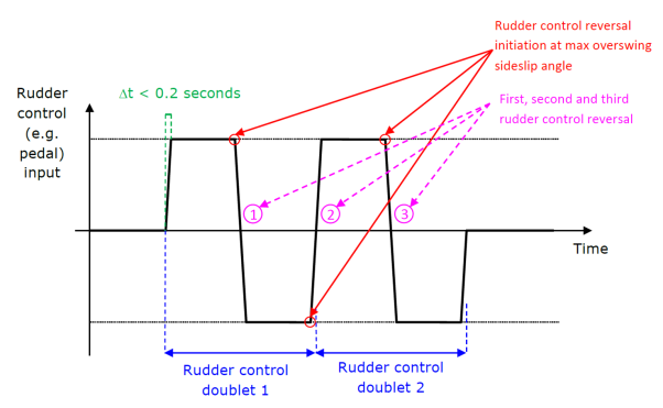
Figure 1: Illustration of the cockpit rudder control inputs

[Amdt No: 25/22]