Signal-in-space models for approach and landing simulation and fault analysis

ED Decision 2022/007/R

1 Purpose

The purpose of this Appendix to the AMC is to provide acceptable signal-in-space models based on known navigation means (facilities external to the aircraft) that can be used to demonstrate in simulation the system performance in approach and landing. It should be noted that system performance depends on the performance of the navigation means (nominal limit and fault), and a performance demonstration conducted using one navigation means may not be valid when using another navigation means due to different nominal limit and fault characteristics.

Note: These models are primarily intended to simulate the characteristics of beams at low altitude and, therefore, the results derived from its use should not be relied on for heights above 150 m (500 ft).

2 ILS CAT I/II/III signal-in-space model

The values given are derived from the performance characteristics for ILS, contained in ICAO Annex 10, Volume I, Sixth Edition, dated July 2006, at Amendment 90, except where otherwise indicated.

ICAO Annex 10 Volume I (Attachment C, paragraph 2.14) defines a standard classification of ILS by using three characters:

(1) facility performance (I, II or III);

(2) ILS points (A, B, C, T, D or E — see definition below) to which the localiser structure conforms to the course structure of a CAT II/III localiser; and

(3) level of integrity and continuity of service (1, 2, 3 or 4).

ILS point ‘A’

A point on the ILS glide path measured along the extended runway centre line in the approach direction at a distance of 7.5 km (4 NM) from the threshold.

ILS point ‘B’

A point on the ILS glide path measured along the extended runway centre line in the approach direction at a distance of 1 050 m (3 500 ft) from the threshold.

ILS point ‘C’

A point through which the downward extended straight portion of the nominal ILS glide path passes at a height of 30 m (100 ft) above the horizontal plane containing the threshold.

ILS reference datum (point ‘T’)

A point at a specified height located above the intersection of the runway centre line and the threshold, and through which the downward extended straight portion of the ILS glide path passes.

ILS point ‘D’

A point 4 m (12 ft) above the runway centre line and 900 m (3 000 ft) from the threshold in the direction of the localiser.

ILS point ‘E’

A point 4 m (12 ft) above the runway centre line and 600 m (2 000 ft) from the stop end of the runway in the direction of the threshold.

Depending on the intended operation, the minimum class of ILS elected will define the detailed characteristics of the ILS to be used for:

—             nominal and limit case analysis;

—             failure cases to be considered; and

—             integrity and continuity analysis.

2.1 Glide path

2.1.1 Glide path angles

It should be assumed that the operationally preferred glide path angle is 3°. The system should be shown to meet all applicable requirements with promulgated glide path angles from 2.5° to 3°. Minimum and maximum glide path angle slopes considered in the demonstrations should be defined and the system should meet all applicable requirements within the defined limits. Where certification is requested for the use of a larger beam angle, the performance on such a beam should be assessed.

—             For CAT I operations, it is recommended to cover at least a 2.5° to 3.5° glideslope range.

—             For CAT II or CAT III operations, it is recommended to cover a 2.5° to 3° glideslope range.

2.1.2 Height of the ILS reference datum (height of glide path at threshold)

For establishing compliance with the longitudinal touchdown performance limits, it may be assumed that the height of the ILS reference datum is 15 m (50 ft).

2.1.3 Glide path alignment accuracy

It should be assumed that the standard deviation of the beam angle about the nominal angle (θ) is 0.025 θ.

2.1.4 Displacement sensitivity

It should be assumed that the angular displacement from the nominal glide path for 0.0875 DDM has the value of 0.12 θ.

2.1.5 Glide path structure

For the purposes of simulation, the noise spectrum of the ILS glide path may be represented by a white noise passed through a low-pass first-order filter of time constant 0.5 s.

Note: For CAT I ILS, a combination of high-frequency and low-frequency noise would be more representative of the actual noise experienced in-service.

For the whole of the approach path, the output of the filter should be set to a two-sigma level of:

—             0.035 DDM up to point ‘C’ for facility performance Type I; and

—             0.023 DDM up to ILS reference datum (point ‘T’) for facility performance Τype II or III.

(Background: An interpretation of Annex 10, Volume I, Section 3.1.5.4.1 and 3.1.5.4.2)

Note 1: ICAO Annex 10 Section 3.1.5.4 defines higher value prior point ‘B’ for Type II or III facilities. Since the model is intended to be used only below 500 ft, the increase value prior point B may not be considered.

Note 2: This model is primarily intended to simulate the characteristics of beams at low altitude and, therefore, the results derived from its use should not be relied on for heights above 150 m (500 ft).

2.1.6 Glide fault mode

The effect of a glideslope malfunction can be modelled as a ramp with a start time, a ramp rate, a glide monitoring threshold and a time-to-alert, as illustrated in Figure 1. As the effect of the glide fault may differ depending on start time and ramp rate, the combination that provides the most severe effect on aircraft deviation shall be considered.

Figure 1: ILS glide malfunction transient

The glide malfunction transient depends on the facility performance type:

	Facility performance Type I	Facility performance Type II or III
Glide monitoring threshold (maximum shift of the mean glide path)	minus 0.075 θ (below nominal glide) plus 0.10 θ (above nominal glide)
Time-to-alert	6 s	2 s

Table 1: Glideslope monitoring threshold and time-to-alert based on facility performance

2.2 Localiser

2.2.1 Course alignment accuracy

It should be assumed that at the threshold the standard deviation of the course line about the centre line is:

—             3.5 m (12 ft) for facility performance Type I; and

—             1.5 m (5 ft) for facility performance Type II or III.

Note: The Type II or III value is between those given in ICAO Annex 10, section 3.1.3.6 for CAT II and CAT III ILS which are assumed to be three-sigma values, 2.5 m (8.3 ft) and 1.0 m (3.3 ft) respectively.

2.2.2 Displacement sensitivity

It should be assumed that the nominal displacement sensitivity at the ILS reference datum (Point ‘T’) has the value of 0.00145 DDM/m.

2.2.3 Course structure

For the purposes of simulation, the noise spectrum of the ILS localisers may be represented by a white noise passed through a low-pass first-order filter of time constant 0.5 s.

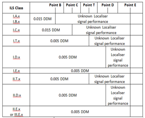
The two-sigma level value of the filter output should be set according to the minimum class of the ILS considered as per the following table:

Note: For CAT I ILS, a combination of high-frequency and low-frequency noise would be more representative of the actual noise experienced in-service.

—             Facility performance Type I: for initial approach path, the output of the filter should be set to a two-sigma level of 0.005 DDM up to the ILS point (A, B, C, T, D or E) elected as the minimum required for the operation.

—             If the minimum required for the operation is ‘A’ or ‘B’, for final approach path, the output of the filter should be set to a two-sigma level of 0.015 DDM up to point ‘C’. After point ‘C’, the localiser signal performance is unknown and should not be used.

—             If the minimum required for the operation is ‘C’, ‘T’, ‘D’ or ‘E’, after the elected point, the localiser signal performance is unknown and should not be used.

—             Facility performance Type II or III: for the whole of the approach path, the output of the filter should be set to a two-sigma level of 0.005 DDM.

2.2.4 Localiser fault mode

The effect of a localiser malfunction can be modelled as a ramp with a start time, a ramp rate, a localiser monitoring threshold and a time-to-alert as illustrated in Figure 2. As the effect of the localiser fault may differ depending on start time and ramp rate, the combination that provides the most severe aircraft deviation shall be considered.

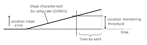
Figure 2: ILS localiser malfunction transient

The localiser malfunction transient depends on the facility performance type:

	Facility performance Type I	Facility performance Type II	Facility performance Type III
Localiser monitoring threshold (maximum shift of the mean course line from the runway centre line)	10.5 m (35 ft)	7.5 m (25 ft)	6 m (20 ft)
Time-to-alert	10 s	5 s	2 s

Table 2: Localiser monitoring threshold and time-to-alert based on facility performance

2.2.5 Integrity and continuity

The probability of radiating false ILS localiser or glide guidance can be assumed to be:

—             for integrity level 1 ILS: no demonstrated values;

—             for integrity level 2 ILS: 1.0 × 10^–7 in any one landing; and

—             for integrity levels 3 & 4 ILS: 0.5 × 10^–9 in any one landing.

The probability of losing the ILS guidance localiser or glide can be assumed to be:

—             for integrity level 1 ILS: no demonstrated values;

—             for integrity level 2 ILS: 4.0 × 10^–6 in any period of 15 s;

—             for integrity level 3 ILS: 2.0 × 10^–6 in any period of 15 s; and

—             for integrity level 4 ILS: 2.0 × 10^–6 in any period of 30 s (localiser) or 15 s (glide).

3 MLS signal-in-space model

The MLS models defined by the ICAO All Weather Operations Panel (AWOP) (reference AWOP/14-WP/659, dated 4/2/93) should be used for approach simulations. Alternatively, if certification of MLS is only sought for ILS lookalike operations, the applicant may use the ILS model defined in paragraph 2. This is based on the assertion that the MLS quality is equal to or better than that of the ILS and requires no further substantiation.

4 GLS signal-in-space model

What follows describes one acceptable model for the assumed characteristics of the GLS guidance errors. Applicants that use an alternate model are responsible for documenting the alternate model, its basis (including a mapping to ICAO Annex 10 characteristics and any additional assumptions made), and its validity.

The ground-based augmentation system (GBAS) performance model simulates the outputs of a fault-free GBAS airborne receiver when used in conjunction with a GBAS ground station categorised as either GAST C or GAST D.

The architecture of the GLS model is illustrated in Figure 3. The GLS model includes a navigation system error (NSE) generator which generates NSEs representative of a GBAS providing approach service type C or D as defined by the applicable requirements [⁵ ICAO Standards and Recommended Practices (SARPs) for the Global Navigation Satellite System (GNSS). Annex 10 to the Chicago Convention, Vol 1., ⁶ RTCA / DO-245, Minimum Aviation System Performance Standards (MASPS) for the Local Area Augmentation System (LAAS)., ⁷ RTCA / DO-253C, Minimum Operational Performance Standards (MOPS) for GPS Local Area Augmentation System (LAAS) Airborne Equipment.]. The position calculator adds NSEs to the true position of the GLS reference point (GRP). The deviation calculator computes the deviations of the GRP given the FAS data. A latency model is applied to each output of the GLS model.

The development of all components of the GLS model is documented in [⁸ ICAO Paper GNSSP-WP-8, Validation of GBAS CAT I Accuracy: A GLS Model and Autoland Simulations for Boeing Airplanes, presented at the ICAO Global Navigation Satellite Systems Panel, Working Group B Meeting, Seattle, WA, May 29 – June 9, 2000.], [⁹ ICAO NSP Mar 2009 WGW/WP 30, SARPS Support for Airworthiness Assessments GLS Signal Modeling, presented by Tim Murphy, Bretigny, 17-27 March 2009.] and [¹⁰ ICAO NSP May 2010 WGW WP 19, SARPS Support for Airworthiness Assessments - More on GLS Signal Modeling, Prepared by Tim Murphy.]. The NSE generator and the NSE step generator are discussed below.

4.1 GBAS NSE generator

The GBAS NSE generator produces NSEs in the along-track, cross-track and vertical directions. The block diagram of the GBAS NSE generator is shown in Figure 4. The Gaussian white noise (GWN) generator produces three independent noise sequences with zero, mean, and unity variance. Each sequence is filtered by a second-order Butterworth filter. The compensation gain which brings the root mean square (rms) of the filtered noise back to unity is obtained as:

 [1]

The filter output is scaled by NSE scale factors K_atrk, K_xtrk, and K_vert. At the beginning of each run, the NSE generator filter should be initialised at a value sampled from a Gaussian distribution consistent with these scale factors.

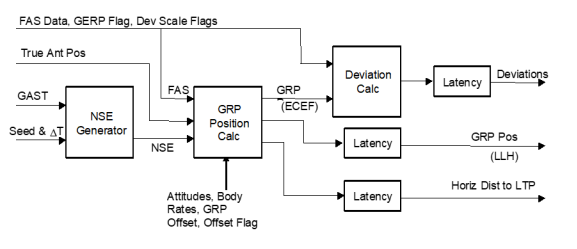
Figure 3: GBAS signal model

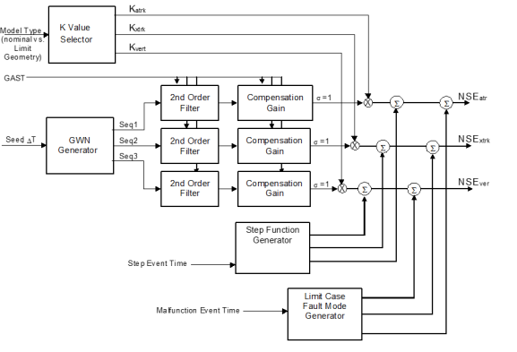
Figure 4: GLS NSE generator

4.2 Second-order filter of GBAS NSE generator

The second-order filter to be implemented in the GBAS NSE generator is characterised by:

 [2]

where ω_n is the natural frequency given by:

—             for GAST C: ω_n = 0.01 rad/s

—             for GAST D: ω_n = 0.033 rad/s

4.3 Noise scale factor

The model accounts for the variation in accuracy due to satellite geometry by setting the noise scale factor to a constant which is sampled from a distribution. For each run, the value of K_vert is determined by selecting a sample, x, from a uniform distribution between 0 and 1. The value of Kvert is then given by the following function of x:

 [3]

where the parameters of the function are dependent on the GBAS approach service type as given in Table 3:

Service type	a1	a1	a3	Kvert_max
GAST C	0.4	0.2	0.006	10 / 5.762 = 1.736
GAST D	0.52	0.47	0.005	10 / 5.762 = 1.736

Table 3: GAST-dependent parameters for Kvert

If the random pick from a distribution between 0 and 1 results in K_vert > K_{vert_max}, then the value should be discarded and another sample should be selected from the uniform distribution set to the maximum value from the table¹¹ This corresponds to the case where VPL > 10 m and, therefore, the system is not available. . An alternative acceptable means for computing the NSE scale factors is given in Section 2 below.

For each run, the value of K_xtrk is determined by selecting a sample, x₁, from a uniform distribution between 0 and 1. For each run, the value of K_atrk is determined by selecting a sample, x₂, from a uniform distribution between 0 and 1. The cross-track and along-track scale factors are then computed by:

 [4]

 [5]

where the parameters of the function are dependent on the GBAS approach service type as given in Table 4:

Service type	a1	a2	a3	Kxtrk_max, Katrk_max
GAST C	0.2	0.1	0.003	40 / 5.762 = 6.942
GAST D	0.21	0.12	0.003	17 / 5.762 = 2.951

Table 4: GAST-dependent parameters for Kxtrk

If the random pick from a distribution between 0 and 1 results in K_xtrk > K_{xtrk_max} or K_atrk > K_{atrk_max}, then the value should be discarded and another sample should be selected from the uniform distribution.

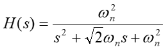
4.4 NSE step generator

The NSE step generator is illustrated in Figure 5. Step errors will occur when individual satellites are removed from the position solution (e.g. a satellite fails and stops transmitting or the user receiver stops tracking a satellite for any reason) or due to an individual satellite rising or setting. The step generator produces representative step errors in the vertical, along-track and cross-track directions. This is accomplished by scaling a unit step function by factors that are derived from representative statistical distributions. First, three random samples, one for each axis, are selected from a zero mean unit variance normal distribution. Then, these samples are multiplied by scale factors that are chosen to simulate the statistical variation in the size of an error that would result from normal variations in the relative geometry between the user and the satellites. Finally, the resultant constant factors are multiplied with a unit step function time sequence.

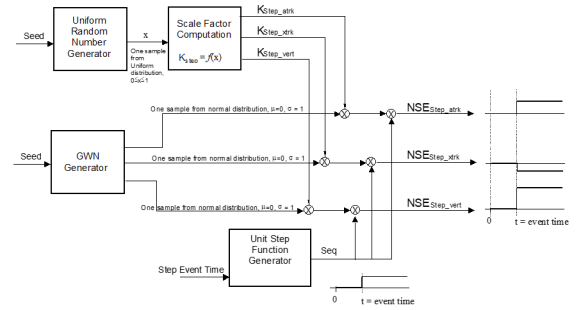
Figure 5: NSE step generator

4.5 NSE step generator scale factor computation

For each run, the value of _{step_vert} is determined by selecting a sample, x, from a uniform distribution between 0 and 1. The value of _{step_vert} is then given by the following function of x:

 [6]

where the parameters of the function are dependent on the GBAS approach service type as given in Table 5:

Service type	b1	b2	b3
GAST C	0.4	0.8	0.07	FASVAL/2
GAST D	0.5	0.8	0.05	3.5

Table 5: GAST-dependent parameters for

If the random pick from a distribution between 0 and 1 results in _{step_vert} > _{step_vert_max}, then the value should be discarded and another sample should be selected from the uniform distribution.

For each run, the value of _{step_xtrk} is determined by selecting a sample, x₁, from a uniform distribution between 0 and 1. The value of _{step_atrk} is determined by selecting a sample, x₂, from a uniform distribution between 0 and 1. The cross-track and along-track NSE step scale factors are then computed by:

  [7]

 [8]

where the parameters of the function are dependent on the GBAS approach service type as given in Table 6:

Service type	b1	b2	b3
GAST C	0.32	0.32	0.05	20 m
GAST D	0.35	0.35	0.35	5.5 m

Table 6: GAST-dependent parameters for or

If the random pick from a distribution between 0 and 1 results in _{step_xtrk} > _{step_xtrk_max}, or _{step_atrk}  > _{step_axtrk_max}, then the value should be discarded and another sample should be selected from the uniform distribution.

4.6 Latency model

The latency of the GLS output should be delayed for a period of 400 ms.

4.7. Fault mode generator

The limit case or fault mode generator is illustrated in Figure 6.

The fault mode generator produces a ramp error with characteristics as illustrated in Figure 7 Malfunction transient. The effect of a malfunction is modelled as a ramp, with a start time, a ramp rate, and a total exposure time, T_max. The maximum value of the ramp depends on the ramp rate and the time-to-alert. The ramp is assumed to increase to the level of the maximum value and then to exceed that value for a period equal to the time-to-detect and mitigate the failure. The erroneous satellite is isolated and the error returns to the nominal value (i.e. the fault error is set to zero). The model may alternatively produce step errors where the maximum change in error due to the step is specified rather than the ramp rate. (See reference [¹² T. Murphy, M Harris, C. Shively, L. Azoulai , M. Brenner, Fault Modeling for GBAS Airworthiness Assessments, Proceedings of the Institute of Navigation Global Navigation Satellite System Conference, 2010.] for more details regarding GLS fault modelling.)

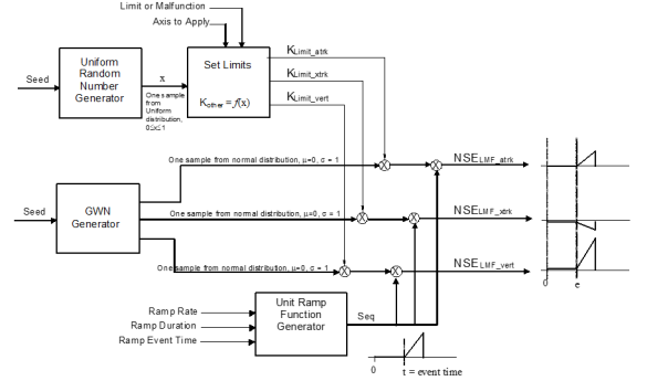
Figure 6: Limit malfunction generator

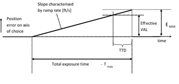
Figure 7: Malfunction transient

From Figure 7, it can be seen that for the ramp:

 [9]

E_MAX and the effective vertical alert limit (VAL) depend on the type of malfunction. For satellite ranging sources, the effective VAL is a function of the maximum error allowable with probability greater than 1 × 10^–9 by the P_md performance constraint with conditional probability (reference [¹³ T. Murphy, M Harris, C. Shively, L. Azoulai , M. Brenner, Fault Modeling for GBAS Airworthiness Assessments, Proceedings of the Institute of Navigation Global Navigation Satellite System Conference, 2010.], Appendix B, Section 3.6.7.3.3.3) (i.e. 1.6 m), multiplied by the geometry screening limit.

  [10]

where is the maximum vertical projection for any satellite allowed by geometry screening.

The aircraft manufacturer limits the size of by specifying a maximum S_vert for satellites used in the position solution as described in reference [¹⁴ M. Harris, T. Murphy, Geometry Screening for GBAS to Meet CAT III Integrity and Continuity Requirements, Proceedings of the Institute of Navigation International Technical Meeting 2007.].

For ground segment reference receiver failures, the effective VAL will depend on the geometry screening applied in the airborne equipment. If no additional geometry screening is applied other than VPL<VAL, the maximum effective VAL is 9.35 [m] (see Table 7 Malfunction transient characteristics in the vertical direction). If additional geometry screening is applied, a lower effective VAL may result. Reference [¹⁵ M. Harris, T. Murphy, Geometry Screening for GBAS to Meet CAT III Integrity and Continuity Requirements, Proceedings of the Institute of Navigation International Technical Meeting 2007.] explains how to compute the effective VAL given additional geometry screening. Error! Reference source not found.Figure 8 Maximum error and T_BAC as a function of alert limits shows a plot of maximum vertical and lateral errors as a function of vertical and lateral alert limit screening. The calculations to produce the plot in Figure 8 are described in detail in reference [¹⁶ Neri, P., Macabiau, C., Azoulai, L., Study of a GBAS Model for CAT II/III Simulations, Proceedings of the 22nd International Technical Meeting of The Satellite Division of the Institute of Navigation (ION GNSS 2009), Savannah, GA, September 2009.].

For ionospheric anomalies, the maximum vertical error E_max is limited to a specified maximum allowable position error for the airborne installation for each axis, vertical (MaxE_V) and lateral (MaxE_L), as a part of the satellite geometry screening in the avionics [¹⁷ Use of GNSS signals and their augmentations for civil Aviation Navigation during Approaches with Vertical Guidance and Precision Approaches – PhD Thesis P. Neri – 2011.]. These values along with broadcast information provided by the ground station determine the geometry screening.

Table 7 and Table 8 give the characteristics for transient errors in the vertical and horizontal directions respectively for each of the three major identified fault types.

Fault type	Service type	Ramp rates [m/s]	Effective VAL [m]	Emax [m]	Time-to-detect (TTD) [s]
Ranging source failures	GAST C	0–	10	Dependent	6
	GAST D	0–	1.6 × Svert	Dependent	2.5
Iono- anomaly	GAST C	0–4	n/a	N/A	n/a
	GAST D	0–4	n/a	MaxEV	n/a
Single-reference receiver failure	GAST C	0–	10	Dependent	6
	GAST D	0–	9.35 [Note]	Dependent	2.5

Table 7: Malfunction transient characteristics in the vertical direction

Note: This value is an absolute worst case assuming no additional geometry screening is afforded based on reference receiver fault monitoring using TBAC. Smaller maximum values can be obtained by using additional geometry screening as per reference [¹⁸ Neri, P., Macabiau, C., Azoulai, L., Study of a GBAS Model for CAT II/III Simulations, Proceedings of the 22nd International Technical Meeting of The Satellite Division of the Institute of Navigation (ION GNSS 2009), Savannah, GA, September 2009.].

Fault type	Service type	Ramp rates [m/s]	Effective LAL [m]	Emax [m]	Time-to-detect (TTD) [s]
Ranging source failures	GAST C	0–	40	Dependent	6
	GAST D	0–	1.6  Slat	Dependent	2.5
Iono- anomaly	GAST C	0–4	n/a	n/a	n/a
	GAST D	0–4	n/a	MaxEL	n/a
Single-reference receiver failure	GAST C	0–	40	Dependent	6
	GAST D	0–	35.9 [Note]	Dependent	2.5

Table 8: Malfunction transient characteristics in the lateral direction

Note: This value is an absolute worst case assuming no additional geometry screening is afforded based on reference receiver fault monitoring using TBAC. Smaller maximum values can be obtained by using additional geometry screening as per reference [¹⁹ Neri, P., Macabiau, C., Azoulai, L., Study of a GBAS Model for CAT II/III Simulations, Proceedings of the 22nd International Technical Meeting of The Satellite Division of the Institute of Navigation (ION GNSS 2009), Savannah, GA, September 2009.].

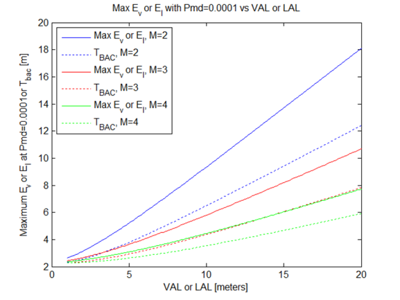
Figure 8: Maximum error and TBAC as a function of alert limits

4.8 Integrity and continuity

The probability of issuing false GLS guidance can be assumed to be:

—             for GAST C: 2.0 × 10^–7 in any one landing; and

—             for GAST D: 1 × 10^–9 in any period of 15 s.

The probability of losing GLS guidance can be assumed to be:

—             for GAST C: 8.0 × 10^–6 in any period of 15 s;

—             for GAST D: 2 × 10^–6 in any period of 15 s.

4.9 Alternative method for calculating and using the NSE model scale factors

4.9.1 Estimation of 10-point piecewise linear interpolation of GBAS NSE — GAST D

An alternative method to use the NSE model is to compute, before launching any run of the Monte Carlo autoland simulations, the distributions of the scale factors, K_vert and K_xtr = K_atrk. For these two last quantities, we conservatively allocate the worst horizontal sigma. These distributions have been computed using assumptions described in [²⁰ Neri, P., Macabiau, C., Azoulai, L., Study of a GBAS Model for CAT II/III Simulations, Proceedings of the 22nd International Technical Meeting of The Satellite Division of the Institute of Navigation (ION GNSS 2009), Savannah, GA, September 2009.] and [²¹ Use of GNSS signals and their augmentations for civil Aviation Navigation during Approaches with Vertical Guidance and Precision Approaches – PhD Thesis P. Neri – 2011.]. Then, for each run of the Monte Carlo simulations, we draw, from these two distributions, a sigma vertical = K_vert and a worst horizontal sigma for K_xtrk and K_atrk, at the beginning of the approach, which are kept constant during the approach.

In order to facilitate the use of these distributions, the 10-point piecewise linear interpolation of K_vert and K_{worst_horizontal_sigma} are provided on the histograms and using a dual entry table X-axis corresponding to sigma_vert or worst_horizontal_sigma in metres.

4.9.2 Sigma vertical

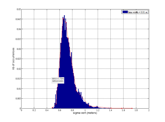
Figure 9: Sigma vertical samples

Sigma_vert	Number of occurrences
0.485000000000000	0.000429191837945
0.543326533206011	0.002257116788039
0.655055242735278	0.045229563598357
0.699018742036146	0.043376936959747
0.731326218889690	0.035448466874264
0.860858976217526	0.008926572687034
1.070145122860493	0.001211926592757
1.409975954322260	0.000073333137778
1.573104102697827	0.000010035060959
1.735000000000000	0.000008491205427

4.9.3 Worst horizontal sigma

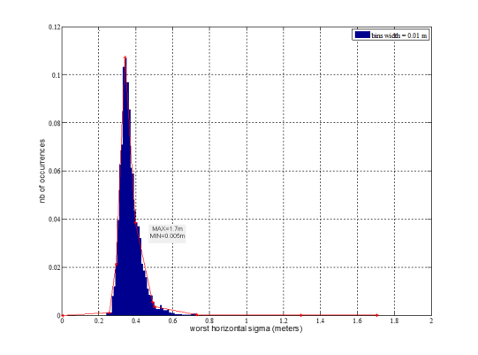
Figure 10: Worst horizontal sigma samples

worst_horizontal_sigma	Number of occurrences
0.005000000000000	0
0.257665870406134	0.001235856353506
0.293780182441118	0.021311381766140
0.341769349550846	0.107172907188037
0.398519584681962	0.038574002399152
0.489966724012817	0.005669037514146
0.501954763905412	0.003652762189125
0.733255508608094	0.000223859052165
1.294724573608414	0.000000771927766
1.705000000000000	0.000000771927766

As with the NSE noise scale factors, an alternative way of using the step function is to derive scale factors sigma_step_vert and worst_sigma_step horizontal to take into account steps induced by the loss of tracking of satellites by the receiver due to geometry (rise/set of satellites) or due to satellite failures. The distributions and the 10-point piecewise linear interpolations are provided below for these two cases for the two dimensions.

4.9.4 Rise/set — sigma step vertical

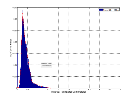
Figure 11: Rise/set sigma samples

Rise/Set Sigma_step_vert	Number of occurrences
0.005000000000000	0.000102160167567
0.072435248412769	0.000251314012215
0.173069321361968	0.007640899466239
0.183661728498818	0.014862132304962
0.266851710720950	0.032471159430220
0.360116883106780	0.022183880145120
0.560386526870370	0.010022935263488
0.707103250848933	0.002542678888367
1.168108921989317	0.000590218235325
1.605000000000000	0

4.9.5 Rise/set — worst sigma step horizontal

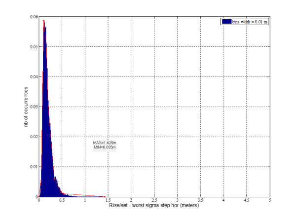
Figure 12: Rise/set worst sigma step horizontal samples

Rise/Set Worst Sigma_Step_Hor	Number of occurrences
0.005000000000000	0.000002897188944
0.041875996448845	0.004326488398194
0.054920944044943	0.005392271389607
0.109250543156205	0.058667264538146
0.163832898257929	0.050878995869548
0.205763067528231	0.030017730600579
0.339826367851692	0.005884118967452
0.481495931510671	0.001622467406624
0.537593983881708	0.001038030498786
1.425000000000000	0.000000090537154

4.9.6 Signal loss — sigma step vertical

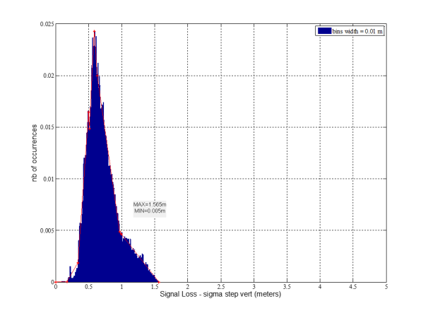
Figure 12: Rise/set worst sigma step horizontal samples

Signal loss Sigma_Step_Vert	Number of occurrences
0.005000000000000	0
0.175788354389016	0.000006172962943
0.341225896607212	0.001849289916083
0.501345966346395	0.016428884464905
0.509272880272156	0.014817130740563
0.585415172749149	0.024277512141267
0.634728223925139	0.019985074857159
0.971964045257760	0.004855442265040
0.993665191757176	0.004618156897366
1.565000000000000	0

4.9.7 Signal loss — worst sigma step horizontal

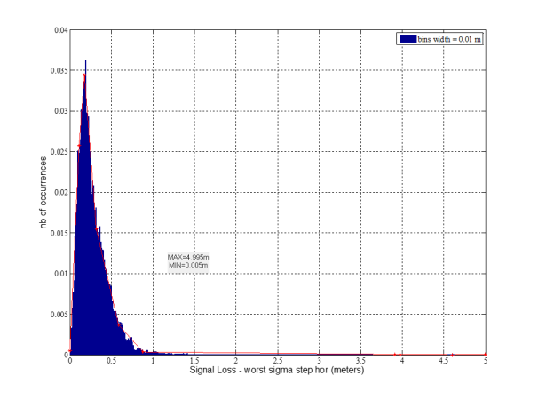
Figure 14: Signal loss worst sigma step horizontal sigma samples

Signal loss worst Sigma_Step_Hor	Number of occurrences
0.005000000000000	0.000476007789371
0.115610839554299	0.025790440689983
0.180148721789614	0.034439075056633
0.320833114781513	0.015472307517217
0.586810140697307	0.003675003851236
0.880744610706960	0.000358424380494
3.908283843494504	0.000000000123437
3.975118428756177	0.000000000123437
4.601736622281720	0
4.995000000000000	0.000000016910875

Wind models for approach and landing simulation

1 Purpose

The purpose of this AMC is to provide acceptable wind, turbulence and wind shear models that can be used to demonstrate in simulation system performance in approach and landing.

2.1 Wind model Number 1

2.1.1 Mean wind

It may be assumed that the cumulative probability of reported mean wind speed at landing, and the crosswind component of that wind are as shown in Figure 15 Cumulative probability of reported mean wind and headwind, tailwind and crosswind components when landing. Normally, the mean wind which is reported to the pilot is measured at a height which may be between 6 m (20 ft) and 10 m (33 ft) above the runway. The models of wind shear and turbulence given in paragraphs 3.2 and 3.3 assume this reference height is used.

2.1.2 Wind shear

2.1.2.1 Normal wind shear

Wind shear should be included in each simulated approach and landing unless its effect can be accounted for separately. The magnitude of the shear should be defined by the expression:

u = 0.43 U log10 (z) + 0.57 U   (1)

where ‘u’ is the mean wind speed at height z metres (z ≥ 1 m) and ‘U’ is the mean wind speed at 10 m (33 ft).

2.1.2.2 Abnormal wind shear

The effect of wind shears exceeding those of paragraph 2.1.2.1 should be investigated using known severe wind shear data.

2.1.3 Turbulence

2.1.3.1 Horizontal component of turbulence

It may be assumed that the longitudinal component (in the direction of mean wind) and lateral component of turbulence may each be represented by a Gaussian process having a spectrum of the form:

() =    (2)

where:

() = a spectral density [[metres/s]² per [radian/metre]]

 = root mean square (rms) turbulence intensity = 0·15 U

L = scale length = 183 m (600 ft)

 = frequency [radians/metre]

2.1.3.2 Vertical component of turbulence

It may be assumed that the vertical component of turbulence has a spectrum of the form defined by equation (2) in paragraph 2.1.3.1.

The following values have been in use:

 = 2.8 km/h (1.5 kt) with L = 9.2 m (30 ft)

or alternatively

 = 0.09 U with L = 4·6 m (15 ft) when z < 9.2 m (30 ft)

and L = 0.5 z when 9.2 < z < 305 m (30 < z < 1 000 ft)

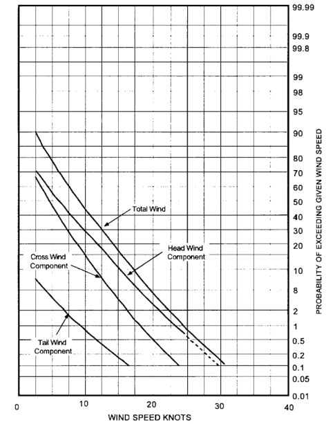
Figure 15: Cumulative probability of reported mean wind and headwind, tailwind and crosswind components when landing

Note: This data is based on worldwide in-service operations of UK airlines (sample size: about 2 000).

These cumulative probabilities could be approximated by a Gaussian distribution with characteristics as below:

Wind in runway axis	Mean	Standard deviation
Crosswind	0 kt	7 kt
Longitudinal wind	7.5 kt head	7.3 kt

2.2 Wind model Number 2

2.2.1 Mean wind

The mean wind is the steady-state wind measured at landing. This mean wind is composed of a downwind component (headwind and tailwind) and a crosswind component. The cumulative probability distributions for these components are provided in Figure 16 Headwind–tailwind description (downwind) and in Figure 17 Crosswind description (crosswind).

Alternatively, the mean wind can be defined with magnitude and direction. The cumulative probability for the mean wind magnitude is provided in Figure 8 Annual per cent probability of mean wind speed equalling or exceeding given values, and the histogram of the mean wind direction is provided in Figure 9 Histogram of the mean wind direction relative to runway heading. The mean wind is measured at a reference altitude of 20 ft above ground level (AGL). The models of the wind shear and turbulence given in Sections 2.2.2 and 2.2.3 assume this reference altitude of 20 ft AGL is used.

2.2.2 Wind shear

When stable and steady horizontal wind blows over the ground surface, terrain irregularities and obstacles such as trees and buildings alter the steady wind near the surface and a boundary layer will cause a form of wind shear. The magnitude of this shear is defined by the following expression:

V_wref = 0.204*V₂₀*ln((h + 0.15)/0.15)

where V_wref is the mean wind speed measured at h ft and V₂₀ is the mean wind speed (ft/s) at 20 ft AGL.

Note: This expression does not represent the violent wind shears created by unstable air mass conditions.

2.2.3 Turbulence

2.2.3.1 Turbulence spectra

The turbulence spectra are of the Von Karman form.

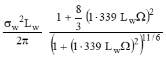
The vertical component of turbulence (perpendicular to the earth’s surface) has a spectrum of the form defined by the following equation:

 = 

The horizontal component of turbulence (in the direction of the mean horizontal wind) has a spectrum of the form defined by the following equation:

 = 

The lateral component of turbulence (perpendicular to the mean horizontal wind) has a spectrum of the form defined by the following equation:

 = 

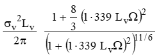
where:

Ω = spectral density [ft/s]²

σ = root mean square (rms) turbulence intensity [ft/s]

L = scale length

Ω = spatial frequency [radians/ft]  = /V_T

ω =  temporal frequency [radians/s]

V_T  =  aircraft speed [ft/s]

2.2.3.2 Turbulence intensities and scale lengths

At or above altitude h1, turbulence is considered to be isotropic, i.e. the statistical properties of the turbulence components are independent. This means that one can consider the turbulence components to have equal intensities.

Below h1, turbulence varies with altitude. In this case, intensity and scale length are expressed as functions of V₂₀ and altitude.

Turbulence intensities

W = 0.1061 V₂₀

where V₂₀ is expressed in kt

where σW is expressed in ft/s

For h < h₁,

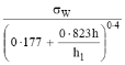
U = V =

For h ≥ h₁,

U = V = W

where h₁ = 1 000 ft

Scale lengths

For h < h₁,

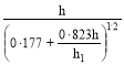
LW = h

L_U = L_V = L_W   = 

For h ≥ h1

L_W   = L_U  = L_V = h₁

where h₁ = 1 000 ft

2.2.3.3 Fixed turbulence intensities for pilot-in-the-loop simulations

The following fixed levels of turbulence intensity [ft/s] have been found to be representative when used to programme low-altitude simulations with the pilot in the loop.

Turbulence intensity	Light	Medium	Heavy
 = v	2.5	5.0	8.3
w	1.25	2.5	4.17

Turbulence scale lengths vary with altitude according to the equations of paragraph 2.2.3.2.

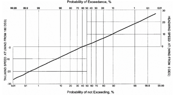
Figure 16: Headwind–tailwind description

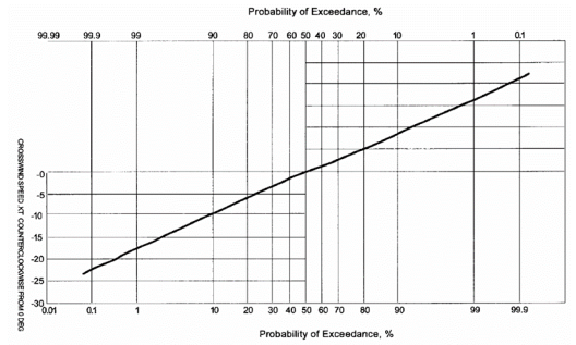
Figure 17: Crosswind description

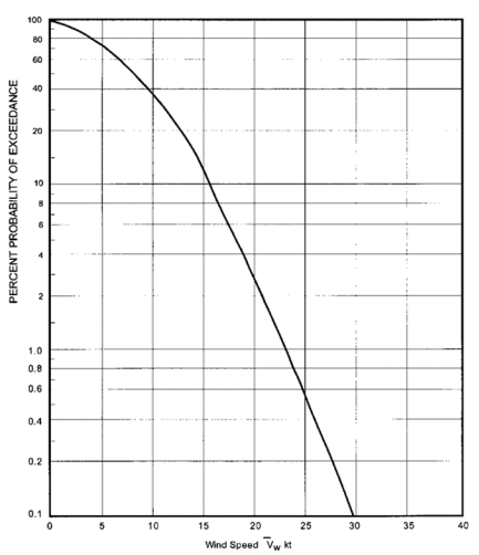
Figure 18: Annual per cent probability of mean wind speed equalling or exceeding given values

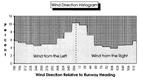
Figure 19: Histogram of the mean wind direction relative to runway heading

2.3. Wind model Number 3

This wind model is a derivative of wind model Number 2. The changes are a result of experience from pilot-in-the-loop simulator tests for Category III HUD certification, where the wind shear and turbulence intensities were found to be more representative.

The changes to wind model Number 2 are as follows:

(a) Paragraph 2.2.2

Change  V_wref  =  0.204 × V₂₀ log n [(h+0.15) ÷ 0.15]

to  V_wref  =  0.165 × V₂₀ log n [(h +0.046) ÷ 0.046]

(b) Paragraph 2.2.3.2

Change  w  =  0.1061 V₂₀

to  w  =  0.0625 V₂₀

where V₂₀ is expressed in kt

where σw is expressed in ft/s

(c) Paragraph 2.2.3.2

Change

Lu to Lu = 600 ft

[Issue: CS-AWO/2]